I was recently flipping through Ross' Simulation (2006, 4th Edition) and saw the following exercise:
Let N be the minimum number of draws from a uniform distribution [until the sum of the variates]exceeds 1. What is the expected value of N? Write a simulation to estimate the expected value.
For example, if v = {0.3, 0.1, 0.5, 0.7, 0.2} is a vector of five random uniform numbers, the value of N for this sample is N=4 because the sum of the first four numbers (0.3+0.1+0.5+0.7) is greater than 1, whereas the sum of the first three number is less than 1. If you choose another set of random numbers, you'll get a different value of N.
The quantity N is a random variable, which is defined by a probability distribution. The expected value of N is the mean of the probability distribution.
Obviously, you need at least two draws from the uniform distribution before the sum of the numbers exceeds 1, since each number is in the open interval (0,1). I thought it would be fun to write a short simulation in SAS/IML software to estimate the distribution of N and its expected value.
The key function to use for this problem is the CUSUM function, which computes a vector that contains the cumulative sums of a vector. If v is the vector defined earlier, then w = CUSUM(v) = {0.3, 0.4, 0.9, 1.6, 1.8}. Another useful trick is transforming the cumulative sums into a logical vector of zeros and ones. For this sample, the logical expression (w<=1) = {1 1 1 0 0} has three 1s, which is the value of N – 1. Putting these two ideas together leads to the following simulation. To show the algorithm clearly, I've written each step on a separate line, rather than combining steps:
proc iml;
/* Define N = max{n : sum_{i=1}^n u_i <= 1. What is E(N)? */
u = j(10000, 10);           /* each sample contains 10 uniform random numbers */
w = j(nrow(u), ncol(u), 0); /* logical matrix of 0s and 1s */
call randseed(1234567);
call randgen(u, "Uniform"); /* fill with uniform numbers */
do i = 1 to nrow(u);
   w[i,] = cusum(u[i,]);    /* compute cumulative sum of each row */
end;
N = (w <= 1)[,+];           /* for each row, how many sum to less than one? */
N = N + 1;                  /* number required to exceed 1 */
EN = mean(N);               /* expected value of N */
print EN;

/* write all values of N to data set and plot distribution */
create Sim var {N}; append; close;
quit;

ods graphics on;
proc freq data=sim;
table N / plots=FreqPlot(scale=percent) nocum;
run; |
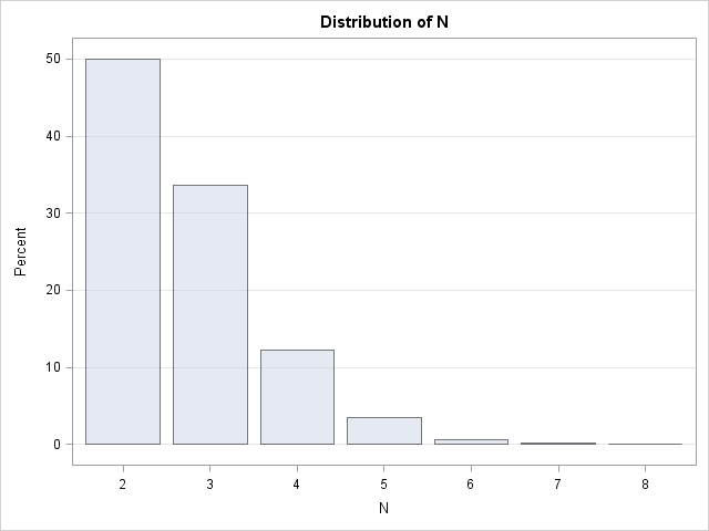
The mean value for this simulation is EN = 2.7206, which turns out to be an estimate for the number e=2.7182818..., the base of the natural logarithm! The probability distribution of N follows the sequence 1/2, 1/3, 1/8, 1/30, .... 1/(k(k – 2)!), and you can show that the expected value of this so-called "uniform sum distribution" is e.
I think that is a pretty cool result! Does anyone know whether there is a geometric argument that explains why e appears in this problem?
I will leave the DATA step version of this problem as an exercise for the motivated reader. Happy computing!

5 Comments
The data step seems way more efficient since you don't need to run every iteration 10 times (not to mention the fact that sometimes it takes more than 10, which I think causes your iml to crash). My way of saving all the counts is probably somewhat inefficient, but it's easy to extend upwards.
data doh (drop=i j sum count) ;
retain sum count mean _2 - _12 ;
array counts[*] _2 - _12 ;
do i=1 to 50000000 ;
sum=0 ;
count=0 ;
do until (sum>1) ;
sum+rand('uniform') ;
count+1 ;
end ;
mean+count ;
do j=2 to dim(counts) ;
if j=count then counts[j-1]+1 ;
end ;
end ;
mean=mean/i ;
output ;
run ;
Yes, I expect that the DATA step will be faster. As I mentioned in my blog, the probability for each k can be computed. P(k>10) is very small (less than 1 in a million), so I didn't need more than 10 elements for the 10,000 draws in my example.
The DATA step could also be written without arrays, if we do not need to show the distribution of the individual values.
data _null_;
simsize=10000;
do i = 1 to simsize;
sum=0;
do j = 1 by 1 until(sum>1);
sum+ranuni(0);
end;
totsum+j;
end;
mean=totsum/simsize;
put mean= simsize=;
run;
I wonder if anything is known about the distribution of the sum that exceeds one? Starting with Art's code above, it seems a beta distribution provides a good fit.
data simsum;
simsize=1E5;
do i = 1 to simsize;
sum=0;
do j = 1 by 1 until(sum>1);
sum+ranuni(0);
end;
output;
end;
run;
proc univariate;
histogram sum / beta(theta=1 scale=1);
run;
Hi,
I wrote a blog post about it which shows how you can arrive at the required result that also provides geometric interpretation.