When I was at SAS Global Forum last week, a SAS user asked my advice regarding a SAS/IML program that he wrote. One step of the program was taking too long to run and he wondered if I could suggest a way to speed it up. The long-running step was a function that finds the largest eigenvalue (and associated eigenvector) for a matrix that has thousands of rows and columns. He was using the EIGEN subroutine, which computes all eigenvalues and eigenvectors—even though he was only interested in the eigenvalue with the largest magnitude.
I asked some questions about his matrix and discovered that it had some important properties:
- The matrix is symmetric, which means that all of its eigenvalues are real.
- The matrix is positive definite, which means that all of its eigenvalues are positive. (Covariance and correlation matrices have this property.)
I told him that the power iteration method is an algorithm that can quickly compute the largest eigenvalue (in absolute value) and associated eigenvector for any matrix, provided that the largest eigenvalue is real and distinct. Distinct eigenvalues are a generic property of the spectrum of a symmetric matrix, so, almost surely, the eigenvalues of his matrix are both real and distinct.
The power iteration method requires that you repeatedly multiply a candidate eigenvector, v, by the matrix and then renormalize the image to have unit norm. If you repeat this process many times, the iterates approach the largest eigendirection for almost every choice of the vector v. You can use that fact to find the eigenvalue and eigenvector.
The power iteration method when the dominant eigenvalue is positive
The power method produces the eigenvalue of the largest magnitude (called the dominant eigenvalue) and its associated eigenvector provided that
- The magnitude of the largest eigenvalue is greater than that of any other eigenvalue. That is, the largest eigenvalue is not complex and is not repeated.
- The initial guess for the algorithm is not an eigenvector for a non-dominant eigenvalue and is not orthogonal to the dominant eigendirection.
It is easy to implement a SAS/IML module that implements the power iteration method for a matrix whose dominant eigenvalue is positive. You can generate a random vector to serve as an initial value for v, or you can use a fixed vector such as a vector of ones. In either case, you form the image A v, normalize that value, and repeat until convergence. This is implemented in the following function:
proc iml;
/* If the power method converges, the function returns the largest eigenvalue.
The associated eigenvector is returned in the first argument, v.
If the power method does not converge, the function returns a missing value.
The arguments are:
v Upon input, contains an initial guess for the eigenvector.
Upon return it contains an approximation to the eigenvector.
A The matrix whose largest eigenvalue is desired.
maxIters The maximum number of iterations.
This implementation assume that the largest eigenvalue is positive.
*/
start PowerMethod(v, A, maxIters);
/* specify relative tolerance used for convergence */
tolerance = 1e-6;
v = v / sqrt( v[##] ); /* normalize */
iteration = 0; lambdaOld = 0;
do while ( iteration <= maxIters);
z = A*v; /* transform */
v = z / sqrt( z[##] ); /* normalize */
lambda = v` * z;
iteration = iteration + 1;
if abs((lambda - lambdaOld)/lambda) < tolerance then
return ( lambda );
lambdaOld = lambda;
end;
return ( . ); /* no convergence */
finish;
/* test on small example */
A = {-261 209 -49,
-530 422 -98,
-800 631 -144 };
v = {1,2,3}; /* guess */
lambda = PowerMethod(v, A, 40 );
if lambda^=. then do;
/* check that result is correct */
z = (A - lambda*I(nrow(A))) * v; /* test if v is eigenvector for lambda */
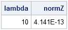
normZ = sqrt( z[##] ); /* || z || should be ~ 0 */
print lambda normZ;
end;
else print "Power method did not converge"; |
Efficiency of the power iteration method
Finding the complete set of eigenvalues and eigenvectors for a dense symmetric matrix is computationally expensive. Multiplying a matrix and a vector is, in comparison, a trivial computation. I know that the power method will be much, much faster, than computing the full eigenstructure, but I'd like to know how much faster. Let's say I have a moderate-sized symmetric matrix. About how much faster is the power method over computing all eigenvectors? To be definite, I'll compare the times for symmetric matrices that have up to 2,500 rows and columns.
I previously have blogged about how to compare the performance of algorithms for solving linear systems. I will use the same technique to compare the performance of the PowerMethod function and the EIGEN subroutine. The following loop constructs a random symmetric matrix for a range of matrix sizes. For each matrix, the program times how long it takes the PowerMethod and EIGEN routines to run:
/***********************************/
/* large random symmetric matrices */
/***********************************/
sizes = do(500, 2500, 250); /* 500, 1000, ..., 2500 */
results=j(ncol(sizes), 3);  /* allocate room for results */
call randseed(12345);
do i = 1 to ncol(sizes);
   n = sizes[i];
   results[i,1] = n;  /* save size of matrix */
   r = j(n*(n+1)/2, 1);
   call randgen(r, "uniform");
   r = sqrvech(r); /* make symmetric */

   q = j(n,1,1);
   t0=time();
   lambda = PowerMethod(q, r, 1000 );
   results[i,2] = time()-t0; /* time for power method */

   t0=time();
   call eigen(evals, evects, r);
   results[i,3] = time()-t0; /* time for all eigenvals */
end;
labl = {"Size" "PowerT" "EigenT"};
print results[c=labl]; |
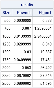
The results are pretty spectacular. The power method algorithm is virtually instantaneous, even for large matrices. In comparison, the EIGEN computation is a polynomial-time algorithm in the size of the matrix. You can graph the timing by writing the times to a data set and using the SGPLOT procedure:
create eigen from results[c=labl]; append from results; close; proc sgplot data=eigen; series x=Size y=EigenT / legendlabel="All Eigenvalues"; series x=Size y=PowerT / legendlabel="Largest Eigenvalue"; yaxis grid label="Time to Compute Eigenvalues"; xaxis grid label="Size of Matrix"; run; |
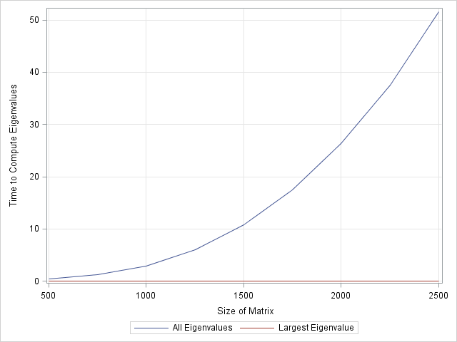
In the interest of full disclosure, the power method converges at a rate that is equal to the ratio of the two largest eigenvalues, so it might take a while to converge if you are unlucky. However, for large matrices the power method should still be much, much, faster than using the EIGEN routine to compute all eigenvalues. The conclusion is clear: The power method wins this race, hands down!
What if the dominant eigenvalue is negative?
If the dominant eigenvalue is negative and v is it's eigenvector, v and A*v point in opposite directions. In this case, the PowerMethod function needs a slight modification to return the dominant eigenvalue with the correct sign. There are two ways to do this. The simplest is to compute z = A*(A*v) until the algorithm converges, and then compute the eigenvalue for A in a separate step. An alternative approach is to modify the normalization of v so that it always lies in a particular half-space. This can be accomplished by choosing the direction (v or -v) that has the greatest correlation with the initial guess for v. I leave this modification to the interested reader.
And to my mathematical friends: did you notice that I used random symmetric matrices when timing the algorithm? Experimentation shows that the dominant eigenvalue for these matrices are always positive. Can anyone point me to a proof that this is always true? Furthermore, the dominant eigenvalue is approximately equal to n/2, where n is the size of the matrix. What is the expected value and distribution of the eigenvalues for these matrices?

25 Comments
Hi Rick, While poking around on your blog, I just read your piece here about the power method applied to random symmetric matrices, with uniform [0,1] entries. Each entry for such a matrix has an expected value of mu= 1/2, and there's a theorem by Furedi and Komlos that implies the largest eigenvalue in this case will be asymptotic to n*mu. That's why you are getting n/2. And the distribution of eigenvalues (except for this largest eigenvalue) will follow the Wigner semicircle law. I ran across these ideas while working on a recent paper -- you can find the Furedi and Komlos reference cited in the following as Ref [3]:
http://www.pnas.org/content/early/2010/12/27/1013213108.full.pdf+html?with-ds=yes
Best wishes, Steve Strogatz
Thanks, Steve! Next week I'm going to blog about simulating these results. You've confirmed the conjectures that the computer experiments suggested were true.
And a very special CONGRATULATIONS for being newly elected to the American Academy of Arts and Sciences! A great and well-deserved honor.
Pingback: The curious case of random eigenvalues - The DO Loop
Hi i am working on a project using the power method and i am having problem in the situation when v and A*v point in the opposite direction.
Could u write the method where the modification should be made and v instead or -v should be used? and vice versa.
Thank you for your time.
The last section discusses some ways to do this. If you need further help, use the SAS/IML Discussion Forum.
I wanted to know the how to calcuate all the eigen values and the eigen vectors.. It is very very imp for the project.... Please help me.
Thanks in Advance..
Thank you and very interesting. But what happens if you have two eigenvalues with equal absolute values? (I'am trying this by hand) Like, if I have this matrix A=[1,0,0;0,0,-1;0,3,0] and start the power method with x=[1;1;1]'.I'm ending up where I'm "running in circles" and I guess the reason is because I have two eigenvalues with equal absolute values. Do you know what it means?
Yes, as Golub and van Loan (1996, 3rd ed, p. 331) say, "the usefulness of the power method depends on the ration |lambda2|/|lambda1|, since it dictates the rate of convergence." You'll never get convergence when the first and second eigenvalues are the same magnitude. In cases like this, you can use a generalization called "orthogonal iteration." See Golub and van Loan, p. 332.
Pingback: 12 Tips for SAS Statistical Programmers - The DO Loop
Hi I am working on a matlab project for the power method and wondering if you could explain to me why i would have for loops in my function such as this one:
for k=1:nmax
z=A*v0;
if abs(max(z))>abs(min(z))
lambda=(max(z));
else
lambda=(min(z));
end
v0=z/lambda;
if k>1 && abs(lambda-lambdaold)
That code is normalizing the vector according to the infinity norm.
hi,
i tried to get the natural timeperiod of a cantilever by eigen value method.. the mathcad/pdf files showing calculation is available in the following link. in mathcad, i am using the command genvals(K,M) & genvecs(K,M) to get the eigen values/eigenvectors for the generalised eigen value prblm.. i converrted the generalised pblm to std eigen format by multiplying throughout by M^-1, and the problm is now [M^-1].[K]-lamda.I=0, which is std eigen format. the eigen values remain same, but vectors are not same.. how do i get the same eigen vectors in standard eigen pblm.. kindly guide
https://drive.google.com/folderview?id=0B9gSrTCMo9R3d3lkeWJnMkZjNzA&usp=sharing
thanks
Hello RICK...i want to know the industrial application of power method in the field of instrumentation and control engg.
plz reply...
What is the minimum number of iterations that should be used for a NxN matrix? (I am using power method for a 154401X154401 matrix)
The method converges according to the ratio r = | lambda_2 | / | lambda_1 |, where lambda_2 is the second largest eigenvalue and lambda_1 is the largest eigenvalue. If the eignevalues are nearly the same magnitude, then the convergence will be slow. If the ratio is small, convergence is fast. In practice, you don't know r, so you should monitor the relative change between successive iterations, as shown in this article, and stop when the relative change is small.
The eigenvectors I am getting are of the order of 10^-6. However even after two successive 100000 iterations, the eigenvectors I get for the maximum eigenvalue does vary.
Relative change means the change in the eigenvalue of the present iteration with respect to the previous iteration?
Yes. In the program the relative change is abs((lambda - lambdaOld)/lambda).
You say "the eigenvectors I get for the maximum eigenvalue" changes from iteration to iteration.
You should verify that the matrix is symmetric so that all eigenvalues are real. If the largest eigenvalue is complex, the power method is useless. Also, see the last section if the largest eigenvalue is negative.
Lastly, you say "the eigenVECTORS ...are of the order of 10^-6." I do not know what that means. Do you mean that the magnitude of the typical element is 1e-6? That makes sense. At each iteration the eigenvector is renormalized so that ||v||=1. Since the vector contains 150k elements, I would not be surprised if a typical element has magnitude of 1e-6.
Yes I meant that the magnitude are of the elements of the eigenvectors are like 2.335e-6, 3.876e-6.
And
The matrix is symmetric, all the eigenvalues are real, and the largest eigenvalue is not complex.
I am trying to calculate the maximum and minimum eigenvalues for a Hamiltonian matrix, which is like
[23 -1 0 0 -1]
[-1 45 -1 0 0]
[ 0 -1 32 -1 0]
[ 0 0 -1 76 -1]
[ -1 0 0 -1 51]
For a small matrix like this, the result converges within 200 iterations. and the values do not vary between two successive simulations.
So that should happen for all hamiltonian matrices, even if they are larger.
So i guess for 150k X 150k matrix, it requires more number of iterations.
I was not considering the relative change, I will have to incorporate it into my code then,
Thanks, for your help.
OK. Good luck. It sounds like you are not using SAS or the code that I provided, so I assume you are coding your own algorithm. Nevertheless, you should read/study what I did and replicate it in your program. Your matrix does not satisfy the traditional definition of a Hamiltonian matrix, but it appears to be banded. You might wish to post your question to math.stackexchange.com and describe your structure. There might be ways to exploit the structure.
Oh. Sorry for the wrong information. The matrix is not Hamiltonian.
I wanted to say it is the matrix obtained from eigenvalue operation of the Hamiltonian Operator in Quantum Mechanics, which I need to solve for getting the eigenvectors. So, I was reffering to this, when I said "Hamiltonian Matrix". I had no idea that Hamiltonian Matrix is actually a different thing. Sorry for that.
I am trying to do the code for this in Python using NumPy and SciPy.
I have one last question.
I calculated the smallest eigenvalue using the Power method by shifting the matrix by lambda_max like B = A - lambda_max * I and then applying power method to B.
I learnt that if the matrix is positive definite, then this works.
However my question is
Can I calculate the other eigenvalues by using a shift like B = A - s*I instead of using the inverse power iteration method because calculating the inverse of a 150k X 150k sparse matrix is not computationally feasible, because inverse of a sparse matrix may or may not be sparse.
You clearly have a lot of questions. I recommend you post to a NumPy discussion forum because I am sure that someone has already written Python code for this.
You have found the largest and smallest eigenvalues by using the power method. You might be able to get the second largest/smallest, but probably not many more. If (lambda, v) is the largest eigenpair, then defining C = A - lambda*v*v` is called "deflation." You can show that the eigenvalues of C are 0 and the nondominant eigenvalues of A. Thus you can apply the power method to C to find the second largest eigenvalue of A. However, a naive implementation of this method is numerically unstable. Google "stability of deflation for eigenvalues." Thus you can rarely continue beyond the second step without losing accuracy.
Thanks, for your help.
I posted on math.stackexchange.com about this.
Here's the link : https://math.stackexchange.com/questions/2626889/finding-the-eigenvalues-between-smallest-and-largest-eigenvalues-of-a-sparse-mat
I guess, I need to study more and try some other method to get this done.
Thanks again.
Learnt that Inverse Power method doesn't require computing the inverse of the matrix. I can now implement it. Thanks for your guidance. :)
Well, I was wrong. I tried running the code multiple times, and saw that the method I said of finding smallest eigenvalue from the Power method by using the shift lambda_max is very unstable. It's better not to use that. Instead using inverse Power method gives very stable results.
I guess the post where I learnt it from, needs some modification -_-
Correction: Not "eigenvalue operation of the Hamiltonian Operator".....
"eigenvalue equation of the Hamiltonian Operator"
From the time-independent Schrodinger's equation:
H. Y = E. Y where Y is the eigenfunction or the wave-function