After my post on detecting outliers in multivariate data in SAS by using the MCD method, Peter Flom commented "when there are a bunch of dimensions, every data point is an outlier" and remarked on the curse of dimensionality. What he meant is that most points in a high-dimensional cloud of points are far away from the center of the cloud.
Distances and outliers in high dimensions
You can demonstrate this fact with a simulation. Suppose that you simulate 1,000 observations from a multivariate normal distribution (denoted MVN(0,Σ)) in d-dimensional space. Because the density of the distribution is highest near the mean (in this case, the origin), most points are "close" to the mean. But how close is "close"? You might extrapolate from your knowledge of the univariate normal distribution and try to define an "outlier" to be any point whose distance from the origin is more than some constant, such as five standardized units.
That sounds good, right? In one dimension, an observation from a normal distribution that is more than 5 standard deviations away from the mean is an extreme outlier. Let's see what happens for high-dimensional data. The following SAS/IML program does the following:
- Simulates a random sample from the MVN(0,Σ) distribution.
- Uses the Mahalanobis module to compute the Mahalanobis distance between each point and the origin. The Mahalanobis distance is a standardized distance that takes into account correlations between the variables.
- Computes the distance of the closest point to the origin.
proc iml;
/* Helper function: return correlation matrix with "compound symmetry" structure:
   {v+v1    v1    v1,
      v1  v+v1    v1,
      v1    v1  v+v1 };   */
start CompSym(N, v, v1);
   return( j(N,N,v1) + diag( j(N,1,v) ) );
finish;
load module=Mahalanobis; /* or insert definition of module here */

call randseed(12345);
N = 1000;                    /* sample size */
rho = 0.6;                   /* rho = corr(x_i, x_j) for i^=j */
dim = T(do(5,200,5));        /* dim=5,10,15,...,200 */
MinDist = j(nrow(dim),1);    /* minimum distance to center */
do i = 1 to nrow(dim);
   d = dim[i];
   mu = j(d,1,0);
   Sigma = CompSym(d,1-rho,rho); /* get (d x d) correlation matrix */
   X = randnormal(N, mu, Sigma); /* X ~ MVN(mu, Sigma) */
   dist = Mahalanobis(X, mu, Sigma);
   MinDist[i] = min(dist);       /* minimum distance to mu */
end; |
The following graph shows the distance of the closest point to the origin for various dimensions.
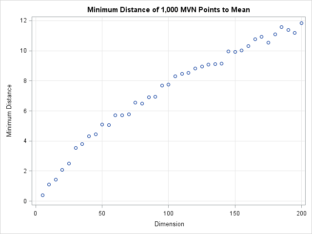
The graph shows that the minimum distance to the origin is a function of the dimension. In 50 dimensions, every point of the multivariate normal distribution is more than 5 standardized units away from the origin. In 150 dimensions, every point is more than 10 standardized units away! Consequently, you cannot define outliers a priori to be observations that are more than 5 units away from the mean. If you do, you will, as Peter said, conclude that in 50 dimensions every point is an outlier.
How to define an outlier cutoff in high dimensions
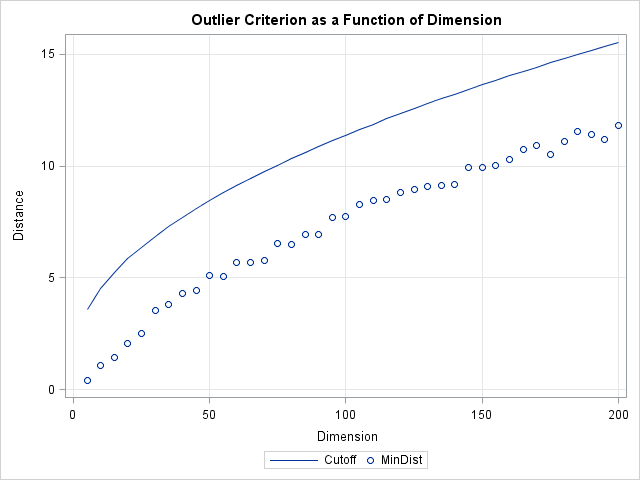
The resolution to this dilemma is to incorporate the number of dimensions into the definition of a cutoff value. For multivariate normal data in d dimensions, you can show that the squared Mahalanobis distances are distributed like a chi-square distribution with d degrees of freedom. (This is discussed in the article "Testing data for multivariate normality.") Therefore, you can use quantiles of the chi-square distribution to define outliers. A standard technique (which is used by the ROBUSTREG procedure to classify outliers) is to define an outlier to be an observation whose distance to the mean exceeds the 97.5th percentile. The following graph shows a the 97.5th percentile as a function of the dimension d. The graph shows that the cutoff distance is greater than the minimum distance and that the two distances increase in tandem.
cutoff = sqrt(quantile("chisquare", 0.975, dim)); /* 97.5th pctl as function of dimension */ |
If you use the chi-square cutoff values, about 2.5% of the observations will be classified as outliers when the data is truly multivariate normal. (If the data are contaminated by some other distribution, the percentage could be higher.) You can add a few lines to the previous program in order to compute the percentage of outliers when this chi-square criterion is used:
/* put outside DO loop */
PctOutliers = j(nrow(dim),1);/* pct outliers for chi-square d cutoff */
...
   /* put inside DO loop */
   cutoff = sqrt( quantile("chisquare", 0.975, d) ); /* dist^2 ~ chi-square */
   PctOutliers[i] = sum(dist>cutoff)/N; /* dist > statistical cutoff */
... |
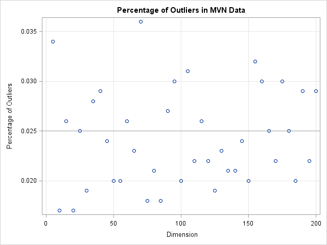
The following graph shows the percentage of simulated observations that are classified as outliers when you use this scheme. Notice that the percentage of outliers is close to 2.5% independent of the dimension of the problem! By knowing the distribution of distances in high-dimensional MVN data, we are able to define a cutoff value that does not classify every point as an outlier.
To conclude, in high dimensions every data point is far away from the mean. If you use a constant cutoff value then you will erroneously classify every data point as an outlier. However, you can use statistical theory to define a reliable rule to detect outliers, regardless of the dimension of the data.
You can download the SAS program used in this article, including the code to create the graphs.

7 Comments
Thanks a lot -- I learned again.I wonder if you can extend this discussion to linear model. I feel many people are interested in detecting outliers/influential points at the linear model setting(with a dependent variable).
Of course. This is essentially what the ROBUSTREG procedure does to detect high leverage points, but it uses robust estimates of location and scale instead of the classical mean and covariance.
Hi Rick
Cool. You can certainly do what you say, and the IML implementation is nice. I don't have time to play with it right now, but will do so ASAP (I hope this weekend).
But, while this definitely shows how to find points that are odder than expected on a given metric (Mahalnobis distance, in this case; clearly you could do something similar for other metrics) if the data are MVN (and, clearly, you could use some other distribution), does this really get at "outlier"?
(Here i am just sort of thinking in public.... these thoughts are fully developed, as will be obvious)
If you have (say) 1000 data points on data with 1000 variables, with some pairs highly correlated and others hardly at all (roughly a problem that I had where I used to work) then you expect 25 or so to be above the cutoff (and, of course, you could pick a different cutoff). But, then, that is what you would *expect*. This is similar to a one-dimensional case - if you sample a LOT of people, then some will be odd; if you sample 100,000 people you might expect to find a 7 foot tall person).
Further (and this could be investigated - or it may be known to theory) how does Mahalnobis distance work when only 1 pair of variables is weird, but neither alone is weird, and the other variables are fine? For example, if you reported that 1 % of people in a general population in the USA were widowed, that wouldn't be weird. And if you said 10 % were under 12 years old, that also wouldn't be weird. But if 0.1 % were widowed *and* under 12, that would be weird! In fact, even in a data set with 100,000 people, you might not expect a single widow under 12 years old.
OK, I'll stop babbling here. :-)
Briefly, there are multivariate outliers and there are univariate (in general, lower-dimensional) outliers. You can have a MV outlier that is not a univariate outlier in any coordinate, such as your 12-year-old widow. You can also have univariate outliers that are not MV outliers.
For highly correlated data, the data will mostly lie in a lower-dimensional subspace. You can use principal components to reduce the dimensionality to a linear subspace. Then you can classify outliers that are within the subspace but away from the center, or you can have outliers that are near the center but are off the subpace. Or both. The geometry of the MV case very rich, indeed.
A nice explanation of what you are trying to explain -- but subject to the restrictive definition of "outlier" that you use ("any point whose distance from the origin is more than some constant"). There is an alternate conception of "outlier" (as "a data point not consistent with the general pattern of the data") that is often more relevant to applications (e.g., for identifying possible measurement errors, data recording errors, or the presence of two or more sub-populations rather than a homogeneous population that can be described by a single nice distribution such a multivariate normal).
Yes. If you know the population distribution you can compute the likelihood that a data point came from the distribution.
Pingback: Monte Carlo estimates of joint probabilities - The DO Loop