A recent discussion on the SAS-L discussion forum concerned how to implement linear interpolation in SAS. Some people suggested using PROC EXPAND in SAS/ETS software, whereas others proposed a DATA step solution.
For me, the SAS/IML language provides a natural programming environment to implement an interpolation scheme. It also provides the flexibility to handle missing values and values that are outside of the range of the data. In this article, I describe how to implement a simple interpolation scheme and how to modify the simple scheme to support missing values and other complications.
Update 04May2020: I have written a more efficient function for performing linear interpolation in SAS. See the newer article about linear interpolation.
What is interpolation?
There are many kinds of interpolation, but when most people use the term "interpolation" they are talking about linear interpolation. Given two points (x1,y1) and (x2,y2) and a value x such that x is in the interval [x1, x2], linear interpolation uses the point-slope formula from high-school algebra to compute a value of y such that (x,y) is on the line segment between (x1,y1) and (x2,y2). Linear interpolation between two points can be handled by defining the following SAS/IML module:
proc iml; /* Interpolate such that (x,y) is on line segment between (x1,y1) and (x2,y2) */ start LinInterpPt(x1, x2, y1, y2, x); m = (y2-y1)/(x2-x1); /* slope */ return( m#(x-x1) + y1 ); /* point-slope formula */ finish; |
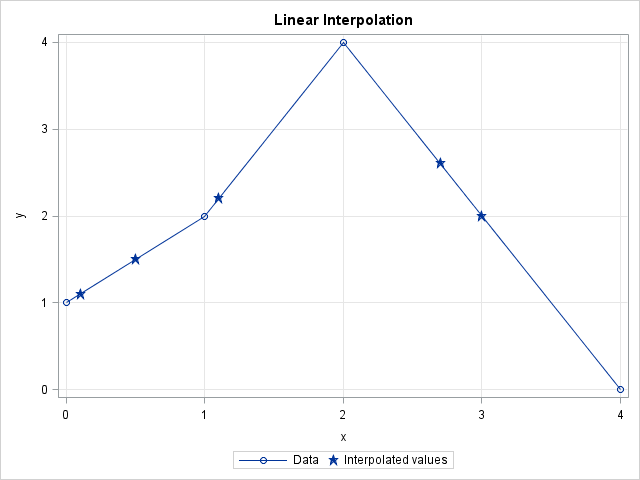
The following graph shows a linear interpolation scheme. The data are shown with round markers. The line segments are the graph of the piecewise-linear interpolation function for the data. Several points (shown with star-shaped markers) are interpolated. The next section shows how to compute the interpolated values.
Linear interpolation: A simple function
Suppose you have a set of points (x1,y1), (x2,y2), ..., (xn,yn) that are ordered so that x1 < x2 < ... < xn. It is not difficult to use the LinearInterpPt function to interpolate a value, v in the interval [x1, xn): you simply find the value of k so that xk ≤ v < xk+1 and then call the LinInterpPt function to interpolate. If you have more than one value to interpolate, you can loop over the values, as shown in the following function:
start Last(x); /* Helper module: return last element in a vector */
return( x[nrow(x)*ncol(x)] );
finish;
/* Linear interpolation: simple version */
start LinInterp1(x, y, v);
/* Given column vectors (x, y), interpolate values for column vector v.
Assume: 1. no missing values in x, y, or v
2. the values of x are unique and sorted
3. each element of v is in the interval [minX, maxX) */
fv = j(nrow(v),1); /* allocate return vector */
do i = 1 to nrow(v);
k = Last( loc(x <= v[i] )); /* largest x less than v[i] */
fv[i] = LinInterpPt(x[k], x[k+1], y[k], y[k+1], v[i]);
end;
return( fv );
finish;
/* test it on some data */
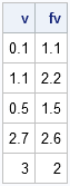
xy = {0 1, 1 2, 2 4, 4 0 };
v = {0.1, 1.1, 0.5, 2.7, 3}; /* interpolate at these points */
fv = LinInterp1(xy[,1], xy[,2], v);
print v fv; |
The elements of v and fv are plotted as stars on the graph in the preceding section. The round markers are the data in the xy matrix.
Linear interpolation: A more robust implementation
The LinearInterp1 function is short, simple, and does the job, but it makes a lot of assumptions about the structure of the (x,y) data and the values to be interpolated. In practice, it is more useful to have a function that makes fewer assumptions and also handles various error conditions. In particular, a useful function would do the following:
- Handle the case where an element of v equals the maximum value xn.
- Handle missing values in x or y by deleting those ordered pairs from the set of data values.
- Check that the nonmissing values of x are unique and issue an error message if they are not. (Alternatively, you could combine repeated values by using the mean or median of the y values.)
- Sort the ordered pairs by x.
- Handle elements of v that are outside of interval [x1, xn]. The simplest scheme is to return missing values for these elements. I do not recommend extrapolation.
start LinInterp(x, y, v);
   /* Assume x and v are sorted and x is unique. Return f(v; x,y)
      where f is linear interpolation function determined by (x,y) */
   fv = j(nrow(v),1); /* allocate return vector */
   begin = 1;         /* set default value */
   idx = loc(v=x[1]); /* 1. handle v[i]=xMin separately */
   if ncol(idx)>0 then do;
      fv[idx] = y[1];
      begin = Last(idx) + 1;
   end;
   do i = begin to nrow(v);      /* remaining values have xMin < v[i] <= xMax */
      k = Last( loc(x < v[i] )); /* largest x less than v[i] */
      fv[i] = LinInterpPt(x[k], x[k+1], y[k], y[k+1], v[i]);
   end;
   return( fv );
finish;

start Interp(_x, _y, _v);
   /* Given column vectors (x, y), return interpolated values of column vector v */
   /* 2. Delete missing values in x and y */
   idx = loc( _x^=. & _y^=. );
   if ncol(idx)<2 then return( j(nrow(_v),1,.) );
   x = _x[idx]; y = _y[idx];

   /* 3. check that the nonmissing values of x are unique */
   u = unique(x);
   if nrow(x)^=ncol(u) then do;
      print "ERROR: x cannot contain duplicate values"; stop;
      /* Alternatively, use mean or median to handle repeated values */
   end;

   /* 4. sort by x */
   xy = x || y;
   call sort(xy, 1);
   x = xy[,1]; y = xy[,2];

   /* 5. don't interpolate outside of [minX, maxX]; delete missing values in v */
   minX = x[1]; maxX = Last(x);
   interpIdx = loc( _v>=minX & _v<=maxX & _v^=. );
   if ncol(interpIdx)=0 then return( j(nrow(_v),1,.) );

   /* set up return vector; return missing for v out of range */
   fv = j(nrow(_v),1,.);
   fv[interpIdx] = LinInterp(x, y, _v[interpIdx] );
   return (fv);
finish;

/* test the modules */
xy = {0 1,  . 3,  2 4,  4 0,  5 .,  1 2};
v = {0.1, 1.1, 0.5, 2.7, 3, ., 4, 5, -1}; /* interpolate at these points */
fv = Interp(xy[,1], xy[,2], v);
print v fv; |
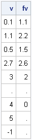
The first five values of v are the same as in the previous section. The last four elements are values that would cause errors in the simple module.
Clearly it takes more work to handle missing values, unordered data, and out-of-range conditions. The simple function with six statements has evolved into two functions with about 30 statements. This is a classic example of "the programmer's 80-20 rule": In a typical program, only 20% of the statements are needed to compute the results; the other 80% handle errors and degenerate situations.
In spite of the extra work, the end result is worth it. I now have a robust module that performs linear interpolation for a wide variety of input data and interpolation values.

4 Comments
On a recent project we used the TIMESERIES procedure to interpolate/transform a set of data into different frequencies. This method does require time-series data to start with, of course, or an easy path to create a date/time identifier in the data. TIMESERIES is part of SAS/ETS, and has the advantage of being able to handle large amounts of data.
In JMP there is the Interpolate function built-in which does this.
Pingback: The difference of density estimates: When does it make sense? - The DO Loop
Pingback: Approximating a distribution from published quantiles - The DO Loop