Most statistical programmers have seen a graph of a normal distribution that approximates a binomial distribution. The figure is often accompanied by a statement that gives guidelines for when the approximation is valid. For example, if the binomial distribution describes an experiment with n trials and the probability of success for each trial is p, then the quantity np(1-p) must be larger than some cutoff (often 5 is used, but sometimes 10) for the approximation to be valid.
The following SAS/IML statements compute the binomial probabilities for n=50 and p=0.8 (so that np(1-p)=8) and for the approximating normal curve, which has mean np and variance np(1-p). These values are plotted by the SGPLOT procedure (SGPLOT statements not shown):
proc iml;
n = 50;  /* number of trials: better approx for 100, 200, etc. */
p = 0.8; /* probability of success for each trial */
mu = n*p;/* classic approximation of binomial pdf by normal pdf */
stddev = sqrt(n*p*(1-p));
xMin = mu - 4*stddev; xMax = mu+4*stddev;
x1 = T(floor(xMin):ceil(xMax)); /* evaluate binomial at integers */
y1 = pdf("Binom", x1, p, n);
x2 = T(do(xMin, xMax, (xMax-xMin)/101));
y2 = pdf("Normal", x2, mu, stddev);
/* write values to SAS data set; plot with SGPLOT */ |
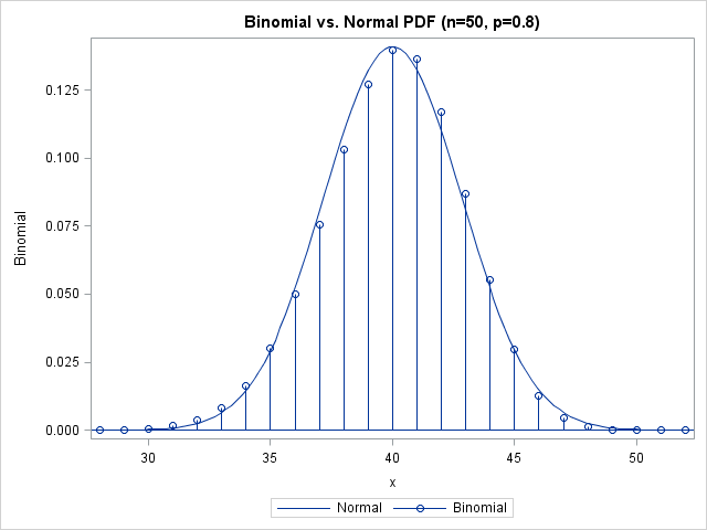
The approximation looks good. However, the figure suggests that you need to be careful if you use a normal distribution to approximate extreme quantiles (such as 0.01 or 0.99) of the binomial distribution. Although the "middles" of the two distributions agree well, there appears to be less agreement in the tails. Also, recall that the quantiles of a discrete distribution are integers, which provides yet another source of error when approximating a binomial quantile with a normal quantile. This is evident when you overlay the normal CDF on the binomial CDF, as in the following figure:
prob = T( do(0.01, 0.99, 0.005) );
q = quantile("binom", prob, p, n);  /* ALWAYS an integer! */
qNormal = quantile("normal", prob, mu, stddev);
diff = q - qNormal; /* error from approximating binomial quantiles */
/* write values to SAS data set; plot with SGPLOT */ |
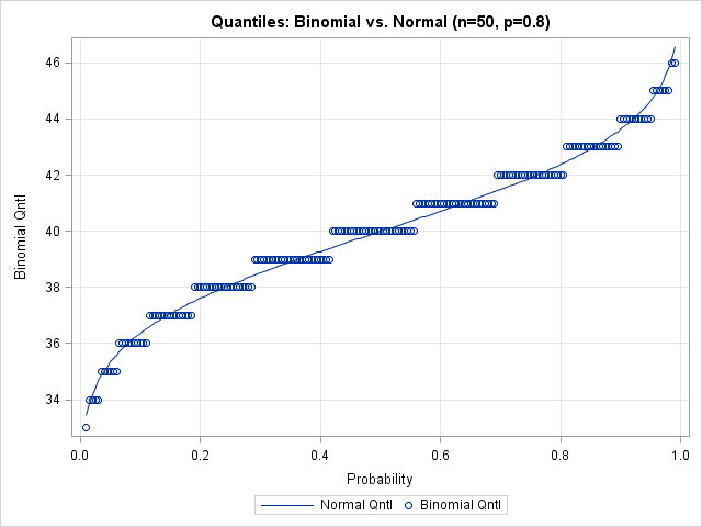
The graph shows that there is considerable error for quantiles near zero and one. Is this important? It can be. For example, if you are creating a funnel plot for proportions the curves on the funnel plot are computed with the quantiles 0.001, 0.025, 0.975, and 0.999. These are extreme quantiles, but they are used to compute the funnel-like control limits, which are the most important feature of the plot. I suspect this is why David Spiegelhalter in his paper "Funnel plots for comparing institutional performance" used a rather complicated formula (in Appendix A.1.1) to interpolate the binomial quantiles in the funnel plot for proportions, rather than using a binomial approximation.
The following graph shows a close-up of the values of the binomial quantiles versus the normal approximation for the extreme quantiles near one. These are the values used to compute the upper control limits in a funnel plot. You can see that the normal approximation exhibits a systematic error, due to differences in the size of the binomial and normal tails.
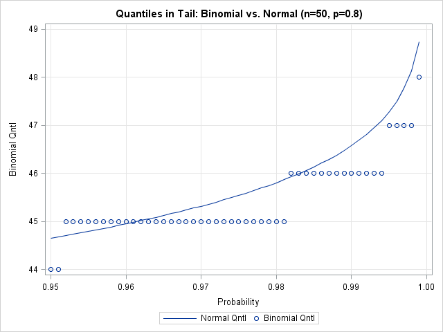
The lesson is this: even though it is common to use a normal distribution to approximate the binomial, the extreme quantiles of the distributions might not be close. Even when np(1-p) is fairly large, there are still sizeable differences in the values of the extreme quantiles of the distributions.

7 Comments
Very interesting and good to know.
Good information but normally ignored...
How much of a difference would the 'continuity correction' make?
That's a good question and I invite you to pursue it. The standard continuity correction shifts the PDF by 1/2 unit, which will also affect the CDF and quantiles. I played around with the idea briefly, but I think it deserves further exploration.
Pingback: Efficient acceptance-rejection simulation: Part II - The DO Loop
I'm new in SAS and would appreciate it if you can provide the codes cor creating the data set and plot. Thanks. Great article!