I work with continuous distributions more often than with discrete distributions. Consequently, I am used to thinking of the quantile function as being an inverse cumulative distribution function (CDF). (These functions are described in my article, "Four essential functions for statistical programmers.")
For discrete distributions, they are not. To quote from my "Four essential functions" article: "For discrete distributions, the quantile is the smallest value for which the CDF is greater than or equal to the given probability." (Emphasis added.)
There is a simple numerical way to examine the relationship between the quantile and CDF: call one function after the other and see if the resulting answer is the same value that you started with. (In other words, compose the functions to see if they are the identity function.) The following SAS/IML statements compute a normal quantile, followed by a CDF:
proc  iml;
/* the quantile function is the inverse CDF for continuous distributions */
prob = 0.8;                   /* start with 0.8 */
q = quantile("Normal", prob); /* compute normal quantile z_0.8 */
cdf = cdf("Normal", q);       /* compute CDF(z_0.8) */
print prob q cdf; /* get back to 0.8 */ |
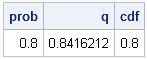
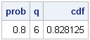
As expected, the QUANTILE function and the CDF function are inverse operations for a continuous distribution such as the normal distribution. However, this is not true for discrete distributions such as the binomial distribution:
/* the quantile function is NOT the inverse CDF for discrete distributions */
prob = 0.8;
q = quantile("Binomial", prob, 0.5, 10); /* q = 80th pctl of Binom(p,n) */
cdf = cdf("Binomial", q, 0.5, 10);       /* CDF(q) does NOT equal 0.8 */
print prob q cdf; |
The reason becomes apparent by looking at the CDF function for the binomial distribution. Consider 10 tosses of a fair coin that has probability p=0.5 of landing on "heads." The Binom(0.5, 10) distribution models this experiment. The CDF function displays the probability that the ten tosses will result in m heads, for m=0, 1, ..., 10, as shown in the following graph:
data BinomCDF(drop=p N);
p = 0.5; N = 10;
do m = 0 to N by 0.1;
   cdf = cdf("Binomial", m, p, N);
   output;
end;
run;

proc sgplot data=BinomCDF;
   title "Probability of m heads in 10 coin tosses";
   title2 "CDF of Binom(0.5, 10)";
   scatter x=m y=cdf;
   xaxis label="Number of Heads" values=(0 to 10) grid;
   yaxis label="P(Number of heads <= m)" grid;
run; |
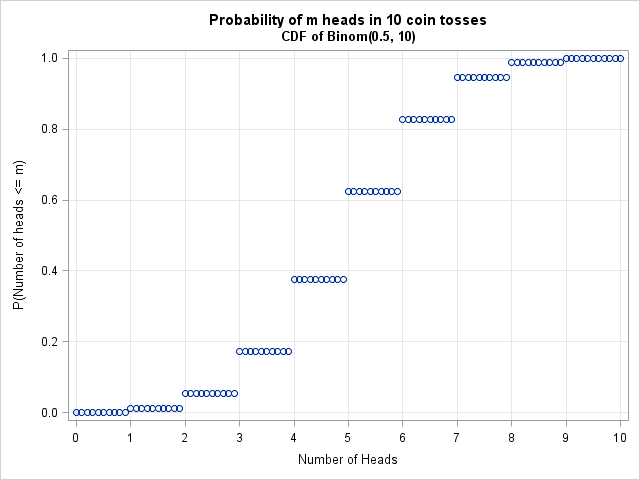
The CDF function is a step function that maps an entire interval to a single probability. For example, the entire interval [5, 6) is mapped to the value 0.623. The quantile function looks similar and maps intervals to the integers 0, 1, ..., 9, 10. For example, the binomial quantile of x is 5 for every x in the interval (0.377, 0.623). This example generalizes: the quantile for a discrete distribution always returns a discrete value.
A consequence of this fact was featured in my article on "Funnel plots for proportions." Step 3 of creating a funnel plot is complicated because it computes a continuous approximation to discrete control limits that arise from binomial quantiles. If you approximate the binomial distribution by a normal distribution, Step 3 becomes simpler to implement, but the funnel curves based on normal quantiles are different from the curves based on binomial quantiles. A future article will explore how well the normal quantiles approximate binomial quantiles.

3 Comments
Pingback: The Normal approximation to the binomial distribution: How the quantiles compare - The DO Loop
Pingback: Fitting a Poisson distribution to data in SAS - The DO Loop
Pingback: Weighted percentiles - The DO Loop