In two previous blog posts I worked through examples in the survey article, "Robust statistics for outlier detection," by Peter Rousseeuw and Mia Hubert. Robust estimates of location in a univariate setting are well-known, with the median statistic being the classical example. Robust estimates of scale are less well-known, with the best known example being interquartile range (IQR), but a more modern statistic being the MAD function.
For multivariate data, the classical (nonrobust) estimate of location is the vector mean, c, which is simply the vector whose ith component is the mean of the ith variable. The classical (nonrobust) estimate of scatter is the covariance matrix. An outlier is defined as an observation whose Mahalanobis distance from c is greater than some cutoff value. As in the univariate case, both classical estimators are sensitive to outliers in the data. Consequently, statisticians have created robust estimates of the center and the scatter (covariance) matrix.
MCD: Robust estimation by subsampling
A popular algorithm that computes a robust center and scatter of multivariate data is known as the Minimum Covariance Determinant (MCD) algorithm. The main idea is due to Rousseeuw (1985), but the algorithm that is commonly used was developed by Rousseeuw and Van Driessen (1999). The MCD algorithm works by sampling h observations from the data over and over again, where h is typically in the range n/2 < h < 3n/4. The "winning" subset is the h points whose covariance matrix has the smallest determinant. Points far from the center of this subset are excluded, and the center and scatter of the remaining points are used as the robust estimates of location and scatter.
This Monte Carlo approach works very well in practice, but it does have the unfortunate property that it is not deterministic: a different random number seed could result in different robust estimates. Recently, Hubert, Rousseeuw, and Verdonck (2010) have published a deterministic algorithm for the MCD.
Robust MCD estimates in SAS/IML software
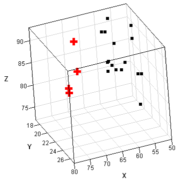
The SAS/IML language includes the MCD function for robust estimation of multivariate location and scatter. The following matrix defines a data matrix from Brownlee (1965) that correspond to certain measurements taken on 21 consecutive days. The points are shown in a three-dimensional scatter plot that was created in SAS/IML Studio.
proc iml;
x = { 80 27 89, 80 27 88, 75 25 90,
62 24 87, 62 22 87, 62 23 87,
62 24 93, 62 24 93, 58 23 87,
58 18 80, 58 18 89, 58 17 88,
58 18 82, 58 19 93, 50 18 89,
50 18 86, 50 19 72, 50 19 79,
50 20 80, 56 20 82, 70 20 91 };
/* classical estimates */
labl = {"x1" "x2" "x3"};
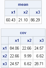
mean = mean(x);
cov = cov(x);
print mean[c=labl format=5.2], cov[r=labl c=labl format=5.2]; |
Most researchers think that observations 1, 2, 3, and 21 are outliers, with others including observation 2 as an outlier. (These points are shown as red crosses in the scatter plot.) The following statement runs the MCD algorithm on these data and prints the robust estimates:
/* robust estimates */ N = nrow(x); /* 21 observations */ p = ncol(x); /* 3 variables */ optn = j(8,1,.); /* default options for MCD */ optn[1] = 0; /* =1 if you want printed output */ optn[4]= floor(0.75*N); /* h = 75% of obs */ call MCD(sc, est, dist, optn, x); RobustLoc = est[1, ]; /* robust location */ RobustCov = est[3:2+p, ]; /* robust scatter matrix */ print RobustLoc[c=labl format=5.2], RobustCov[r=labl c=labl format=5.2]; |
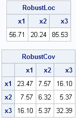
The robust estimate of the center of the data is not too different from the classical estimate, but the robust scatter matrix is VERY different from the classical covariance matrix. Each robust estimate excludes points that are identified as outliers.
If you take these robust estimates and plug them into the classical Mahalanobis distance formula, the corresponding distance is known as the robust distance. It measures the distance between each observation and the estimate of the robust center by using a metric that depends on the robust scatter matrix. The MCD subroutine returns distance information in a matrix that I've called DIST (the third argument). The first row of DIST is the classical Mahalanobis distance. The second row is the robust distance, which is based on the robust estimates of location and scatter. The third row is an indicator variable with the value 1 if an observation is closer to the robust center than some cutoff value, and 0 otherwise. Consequently, the following statements find the outliers./* rules to detect outliers */ outIdx = loc(dist[3,]=0); /* RD > cutoff */ print outIdx; |

The MCD algorithm has determined that observations 1, 2, 3, and 21 are outliers.
Incidentally, the cutoff value used by MCD is based on a quantile of the chi-square distribution because the squared Mahalanobis distance of multivariate normal data obeys a chi-square distribution with p degress of freedom, where p is the number of variables. The cutoff used is as follows:cutoff = sqrt( quantile("chisquare", 0.975, p) ); /* dist^2 ~ chi-square */ |
In a recent paper, Hardin and Rocke (2005) propose a different criterion, based on the distribution of robust distances.
Robust MCD estimates in SAS/STAT software: How to "trick" PROC ROBUSTREG
The ROBUSTREG procedure can also compute MCD estimates. Usually, the ROBUSTREG procedure is used as a regression procedure, but you can also use it to obtain the MCD estimates by "inventing" a response variable. The MCD estimates are produced for the explanatory variables, so the choice of a response variable is unimportant. In the following example, I generate random values for the response variable.
In a regression context, the word "outlier" is reserved for an observation for which the value of the response variable is far from the predicted value. In other words, in regression an outlier means "far away (from the model) in the Y direction." In contrast, the ROBUSTREG procedure uses the MCD algorithm to identify influential observations in the space of explanatory (that is, X) variables. These are also called high-leverage points. They are observations that are far from the center of the X variables. High-leverage points are very influential in ordinary least squares regression, and that is why it is important to identify them.
To generate the MCD estimates, specify the DIAGNOSTICS and the LEVERAGE(MCDINFO) options on the MODEL statement, as shown in the following statements:
/* write data from SAS/IML (or use a DATA step) */ create X from x[c=labl]; append from x; close; quit; data X; set X; y=rannor(1); /* random response variable */ run; proc robustreg data=X method=lts seed=54321; model y = x1 x2 x3 / diagnostics leverage(MCDInfo); ods select MCDCenter MCDCov Diagnostics; ods output diagnostics=Diagnostics(where=(leverage=1)); run; proc print data=Diagnostics; var Obs Mahalanobis RobustDist Leverage; run; |
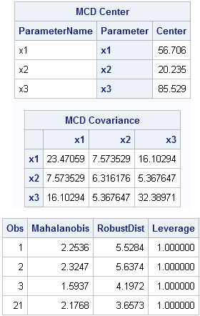
The robust estimates of location and scatter are the same, as are the robust distances. The "leverage" variable is an indicator variable that tells you which observations are far from the center of the explanatory variables. They are multivariate "outliers" in the the space of the X variables, although they are not necessarily outliers for the response (Y) variable.

26 Comments
Good stuff!
When there are a bunch of dimensions, every data point is an outlier .... it might make a good post to talk about the "curse of dimensionality".
Pingback: What is Mahalanobis distance? - The DO Loop
Pingback: The curse of dimensionality: How to define outliers in high-dimensional data? - The DO Loop
Pingback: How to compute Mahalanobis distance in SAS - The DO Loop
Pingback: Popular! Articles that strike a chord with SAS users - The DO Loop
Mentioning "curse of dimensionality": how can I simulate the distance convergence of (dist_max-dist_min)/dist_min -> 0 like mentioned in http://en.wikipedia.org/wiki/Curse_of_dimensionality?
Sorry, but that paragraph is poorly written. Distances between what? And what is being held constant as n-->infinity? I don't understand what they are trying to say.
This data analysis is incorrect. The data results from Rousseeuw's Minvol (Minimum Volume Ellipsoid) is presented , not the Rousseeuw MCD data results.
I don't understand your comment. This article presents the results of an MCD analysis of the Brownlee stackloss data. Can you explain why you say it is incorrect?
Yes, you can also analyze these data by using the MVE method. The SAS/IML chapter about robust statistics provides a comparison of the MVE and MCD methods applied to these data. Researchers have used these data to compare many different analyses.
I used the FORTRAN (source) programs downloaded directly from the Rousseeuw website. The source was compiled (Intel; Lahey/Fujitsu).
Results from Minvol (MVE) Results from fastMCD:
1 2.254 5.528 1 2.2536 12.17328
2 2.325 5.637 2 2.32474 12.25568
3 1.594 4.197 3 1.59371 9.26399
21 2.177 3.657 21 2.17676 7.62277
Since this dataset is small, the fastMCD algorithm will calculate the exact MCD.
Note that the corresponding scatter plots look substantially different from each other.
Yes, I get those exact same numbers for the MD and RD of those observations when I use Rousseeuw's default values for the MVE and MCD routines.
I guess that I need to clarify my previous statements.Your last three' tables' are labeled MCD Center, MCD Covariance, and the third has no label. A novice reader may erroneously conclude that the last 'table' contains the results of the MCD analysis. It does not, but rather contains the results of a MVE analysis. For the sake of clarity, you should probably either replace the data with the actual MCD numbers or label it as the results of a MVE analysis. Hope this clarifies what I was trying to say earlier; I didn't mean to cause any confusion.
Your kind cooperation in this matter is most gratefully appreciated.
All of the tables are from MCD. The column labeled "RobustDist" is the robust MCD distance. I suspect that the source of the discrepancy is that I am not using the default value of h. If you have further questions, post them to the SAS Statistical Community.
Hi Rick, thanks for a very interesting article.
Based on this example I used MCD in IML with time series of interest rate changes. It works fine in this multivariate setting.
However, when I reduce data to only a single time series I experienced that MCD results in strange numbers. The covariance matrix is of course 1x1 and should contain the robust variance. But it is nowhere near the scale of the data squared. For my data, a traditional (non-robust) variance would be 6400, but the MCD value becomes 2.4E-213
In a multivariate setting, MCD provides diagonal elements in the robust covariance matrix that are on a scale similar to the non-robust variances. So it seems that something goes wrong when running MCD on only a single variable.
Do you have any experience in using MCD against a single series and, if so, are there any options that should be set differently ?
Thanks,
JB
MCD and MVE are multivariate methods that require at least two dimensions. For robust univariate estimates of scale, see the article "Detecting outliers in SAS: Part 2: Estimating scale."
Dear Rick,
You said for the robustreg procedure that "he choice of a response variable is unimportant".
Why when I modify the seed number (put y=rannor(2) for example) the results change?
Thank you for your answer.
Samir
Thanks for writing. The ROBUSTREG procedure does two things: (1) it finds high-leverage points among the explanatory variables (the X variables), and (2) it finds outliers among the response values and solves a robust regression problem. This article is about (1) and those estimates depend only on the explanatory variables, so the response doesn't matter for forming those estimates. (Other ROBUSTREG output might change.) However, the estimation process itself (for LTS and M-estimation) uses random subsets of the data, so the estimates could change because of the subsets that are examined. You can add a seed value (for example, SEED=54321) to the PROC ROBUSTREG statement to ensure that the subsets are the same every time that you run the procedure.
Dear Rick,
I remove my question, what change is only the leverage and the outlier detection flag.
Krs,
Samir
Thank you very much Rick!
Your post helped me a lot.
Samir
Hi Rick
If I'm understanding correctly, the obs 1,2,3 and 21 (from the last example) highlight which "records" are influential. This is a big step forward, but work would still need to be done to identify which variable(s) of those records are causing the influence. And of course, this varies from record to record. In my workplace with millions of records and hundreds of variables, health sector, this would not be a trivial exercise. What would you recommend to identify what values were "unusual" from those selected to be "bad leverage points" in any given record? Deviations from each record against the robust mean vector?
Brett
In high dimensions, outliers often have reasonable values in all coordinates. There does not need to be a set of "unusual" values that you can detect. Rather, it is the combination of values across all variables that causes the observation to be an outlier. For example, 140 is a high, but not alarming, value for systolic BP. Similarly, 55 is a low, but not alarming, value of diastolic BP. But a patient whose BP is 130 over 55 is probably an outlier because diastolic and systolic BP tends to be correlated.
Pingback: The Theil-Sen robust estimator for simple linear regression - The DO Loop
Hi Rick,
very interesting and useful tips for outlier identification. Seems to work beautifully, but I'm not sure what the number of leverage points means. SAS help says that the point is declared as a leverage point if the robust distance exceeds what would expected if they were chi-square distributed. If you have more outliers than the cutoff-alpha would indicate, does that mean you have heavier tails than in a multivariate standard normal distribution?
Yes. The robust covariance matrix is used to compute the robust distance, so the assumption that the distances are chi-squared is that the data are MVN from a population with that covariance structure. The large distances might indicate isolated outliers. Alternatively, the assumption might be wrong and you are actually dealing with tails that are heavier than expected under the normality assumption.
Just seeing this for the first time today, almost 10 years after it was written! This is great, I am stealing the IML code for my own diabolical purposes! Thanks, Rick!
Thanks for writing. You cannot steal that which is freely given. Enjoy. I hope you find it useful.