In a previous post, I described how to compute means and standard errors for data that I want to rank. The example data (which are available for download) are mean daily delays for 20 US airlines in 2007.
The previous post carried out steps 1 and 2 of the method for computing confidence intervals for rankings, as suggested in Marshall and Spiegelhalter (1998):
- Compute the mean delay for each airline in 2007.
- Compute the standard error for each mean.
- Use a simulation to compute the confidence intervals for the ranking.
This post carries out step 3 of the method.
Ordering Airlines by Mean Delays
To recap, here is the SAS/IML program so far. The following statements compute the mean delays and standard errors for each airline in 2007. The airlines are then reordered by their mean delays:
proc iml;
/** read mean delay for each day in 2007
    for each airline carrier **/
Carrier = {AA AQ AS B6 CO DL EV F9 FL HA
           MQ NW OH OO PE UA US WN XE YV};
use dir.mvts;
read all var Carrier into x;
close dir.mvts;
meanDelay = x[:,];

/** sort descending; reorder columns **/
call sortndx(idx, MeanDelay`, 1, 1);
Carrier = Carrier[,idx];
x = x[,idx];
meanDelay = meanDelay[,idx]; |
Ranking Airlines...with Confidence
You can use the simulation method suggested by Marshall and Spiegelhalter to compute confidence intervals for the rankings. The following statements sample 10,000 times from normal distributions. (I've previously written about how to write an efficient simulation in SAS/IML software.) Each of these samples represents a potential realization of the underlying random variables:
/** simulation of true ranks, according to the method
    proposed by Marshall and Spiegelhalter (1998)
    British Med. J. **/
/** parameters for normal distribution of means **/
mean = meanDelay`;
sem = sqrt(var(x)/nrow(x)); /** std error of mean **/

p = ncol(Carrier);
NSim = 10000;
s = j(NSim, p); /** allocate matrix for results **/
z = j(NSim, 1);
call randseed(1234);
do j = 1 to p;
   call randgen(z, "Normal", mean[j], sem[j]);
   s[,j] = z;
end; |
The matrix s contains 10,000 rows and 20 columns. Each row is a potential set of means for the airlines, where the ith mean is chosen from a normal distribution with population parameters μi and σi. Because the population parameters are unknown, Marshall and Spiegelhalter advocate replacing the population means with the sample means, and the population standard deviations by the sample standard errors. This kind of simulation is similar to a parametric bootstrap.
The following statements use the SAS/IML RANK function to compute the rank (1–20) for each simulated set of means. (If you need to conserve memory, you can re-use the s matrix to store the ranks.)
/** for each sample, determine the rankings **/ r = j(NSim, p); do i = 1 to NSim; r[i,] = rank(s[i,]); end; |
Each column of the r matrix contains simulated ranks for a single airline. You can use the QNTL subroutine to compute 95% confidence intervals for the rank. Basically, you just chop off the lower and upper 2.5% of the simulated ranks. (If you have not upgraded to SAS/IML 9.22, you can use the QNTL module for this step.)
/** find the 95% CI of the rankings **/
call qntl(q, r, {0.025 0.975}); |
The simulation is complete. The matrix q contains two rows and 20 columns. The first row contains the lower end of the 95% confidence limits for the ranks; the second row contains the upper limit.
You can print q to see the results in tabular form. I prefer graphical displays, so the following statements create a SAS data set that contains the estimated ranks and the upper and lower confidence limits.
d = rank(mean) || T(q);
varNames = {"Rank" "LCL" "UCL"};
create Rank from d[r=Carrier c=varNames];
append from d[r=Carrier];
close Rank; |
It is now straightforward to use SCATTER statement in PROC SGPLOT to create a scatter plot with confidence intervals (called "error bars" in some disciplines):
proc sgplot data=Rank noautolegend; title "Ranking Airlines (On-Time Performance, 2007)"; scatter y=carrier x=Rank / xerrorlower=LCL xerrorupper=UCL; xaxis label="Rank with 95% Confidence Intervals"; yaxis grid discreteorder=data label="Carrier"; run; |
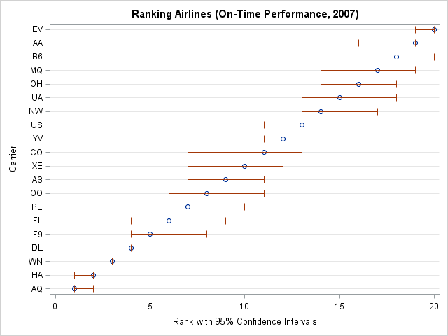
For these data, the ranking of the first three airlines (AQ, HA, WN) seems fairly certain, but there is more uncertainty for the rankings of airlines that are in the middle of the pack. So, for example, if Frontier Airlines (F9) issues a press release about their 2007 on-time performance, it shouldn't claim "We're #5!" Rather, it should state "We're #5 (maybe), but we might be as high as #4 or as low as #8."
In keeping with my New Year's Resolutions, I've learned something new. Next time I want to rank a list, I will pay more attention to uncertainty in the data. Plotting confidence intervals for the rankings is one way to do that.

11 Comments
Should call qntl(q, r, {0.25, 0.975}) be call qntl(q, r, {0.025, 0.975})?
Yes! Thanks so much for finding that typo.
Rick:
A couple more 'issues' arose as I was trying to duplicate this code. First, the third argument to qntl() that you addressed in the previous comment should not contain a comma so that it represents a row vector rather than a column vector.
Finally, I did not find a function var() for a matrix needed to calculate the standard error of the mean for each airline's arrival times. So I manufactured my own:
dev = x - meanDelay;
varx = dev[##,]/(nrow(x)-1);
Sorry for the confusion. The commas are needed for the QNTL function in SAS/IML 9.22 (which I am using), but you are correct that you should use a row vector if you are calling the QNTL module.
The VAR function is another 9.22 feature, and I forgot to point that out.
Pingback: How to sample from independent normal distributions - The DO Loop
Pingback: How to rank values - The DO Loop
Pingback: Computing the variance of each column of a matrix - The DO Loop
Pingback: Funnel plots: An alternative to ranking - The DO Loop
Pingback: Readers’ choice 2011: The DO Loop’s 10 most popular posts - The DO Loop
Pingback: Ranking with confidence: Part 1 - The DO Loop
Pingback: A comparison of different weighting schemes for ranking sports teams - The DO Loop