One of my New Year's resolutions is to learn a new area of statistics. I'm off to a good start, because I recently investigated an issue which started me thinking about spatial statistics—a branch of statistics that I have never formally studied.

During the investigation, I asked myself: Given an configuration of points in a rectangle, how can I compute a statistic that indicates whether the configuration is uniformly spread out in the region?

One way to investigate this question is to look at the density of points in the configuration. Are the points spread out or clumped together?

Binning the Points

In the one-dimensional case, you can use a histogram to visually examine the density of univariate data. If you see that the heights of the bars in each bin are roughly the same height, then you have visual evidence that the data are uniformly spaced.

Of course, you don't really need the histogram: the counts in each bin suffice. You can divide the range of the data into N equally spaced subintervals and write SAS/IML statements that count the number of points that fall into each bin.

It is only slightly harder to compute the number of point that fall into bins of a two-dimensional histogram or, equivalently, into cells of a two-dimensional grid:

1. For each row in the grid...
2. Extract the points whose vertical coordinates indicate that they are in this row. (Use the LOC function for this step!)
3. For these extracted points, apply the one-dimensional algorithm: count the number of points in each horizontal subdivision (column in the grid).

proc iml;
/** Count the number of points in each cell of a 2D grid.
    Input: p    - a kx2 matrix of 2D points
           XDiv - a subdivision of the X coordinate direction
           YDiv - a subdivision of the Y coordinate direction
    Output: The number of points in p that are contained in 
            each cell of the grid defined by XDiv and YDiv. **/
start Bin2D(p, XDiv, YDiv);
   x = p[,1];       y = p[,2];
   Nx = ncol(XDiv); Ny = ncol(YDiv);
 
   /** Loop over the cells. Do not loop over observations! **/
   count = j(Ny-1, Nx-1, 0); /** initialize counts for each cell **/
   do i = 1 to Ny-1; /** for each row in grid **/
      idx = loc((y >= YDiv[i]) & (y < YDiv[i+1]));
      if ncol(idx) > 0 then do;
         t = x[idx]; /** extract point in this row (if any) **/
         do j = 1 to Nx-1; /** count points in each column **/
            count[i,j] = sum((t >= XDiv[j]) & (t < XDiv[j+1]));
         end;
      end;
   end;
   return( count );
finish;

Testing the Binning Module

A convenient way to test the module is to generate 100 random uniform points in a rectangle and print out the counts. The following example counts the number of points in each of 20 bins. There are five bins in each horizontal row and four bins in each vertical column.

call randseed(1234);
p = j(100,2);
call randgen(p, "uniform"); /** 100 random uniform points **/
 
/** define bins: 5 columns and 4 rows on [0,1]x[0,1] **/
XMin = 0; XMax = 1; dx = 1/5;
YMin = 0; YMax = 1; dy = 1/4;
XDiv = do(XMin, XMax, dx);
YDiv = do(YMin, YMax, dy);
 
count = Bin2D(p, XDiv, YDiv);

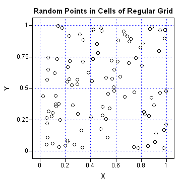
A visualization of the random points and the grid is shown in the scatter plot. From the graph, you can quickly estimate that each bin has between 1–10 points. The exact counts are contained in the count matrix.

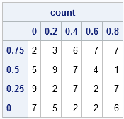
Notice that the Y axis of the scatter plot has large values of Y at the top of the image and small values at the bottom of the image. In order to compare the values of the count matrix with the scatter plot, it is helpful to reverse the order of the rows in count:

/** reverse rows to conform to scatter plot **/
count = count[nrow(count):1,];
c = char(XDiv, 3); /** form column labels **/
r = char(YDiv[ncol(YDiv)-1:1], 4); /** row labels (reversed) **/
print count[colname=c rowname=r];

You can use these bin counts to investigate the density of the point pattern. I'll present that idea on Friday.