A customer asks if it is possible to put one graph inside of another. The question states that this format is sometimes used in the New England Journal of Medicine. Click here to see the original question in SAS Communities and the graph. There are several ways of inserting graphs into graphs. I will illustrate three. See Lelia McConnell's post Picture-in-Picture for a fourth method. The three methods that I show all have in common that you can store a graph in an image file and then use SG Annotation (or its GTL equivalent) to display that graph in conjunction with another graph. See Dan Heath's PharmaSUG paper Now You Can Annotate Your GTL Graphs! for more information.
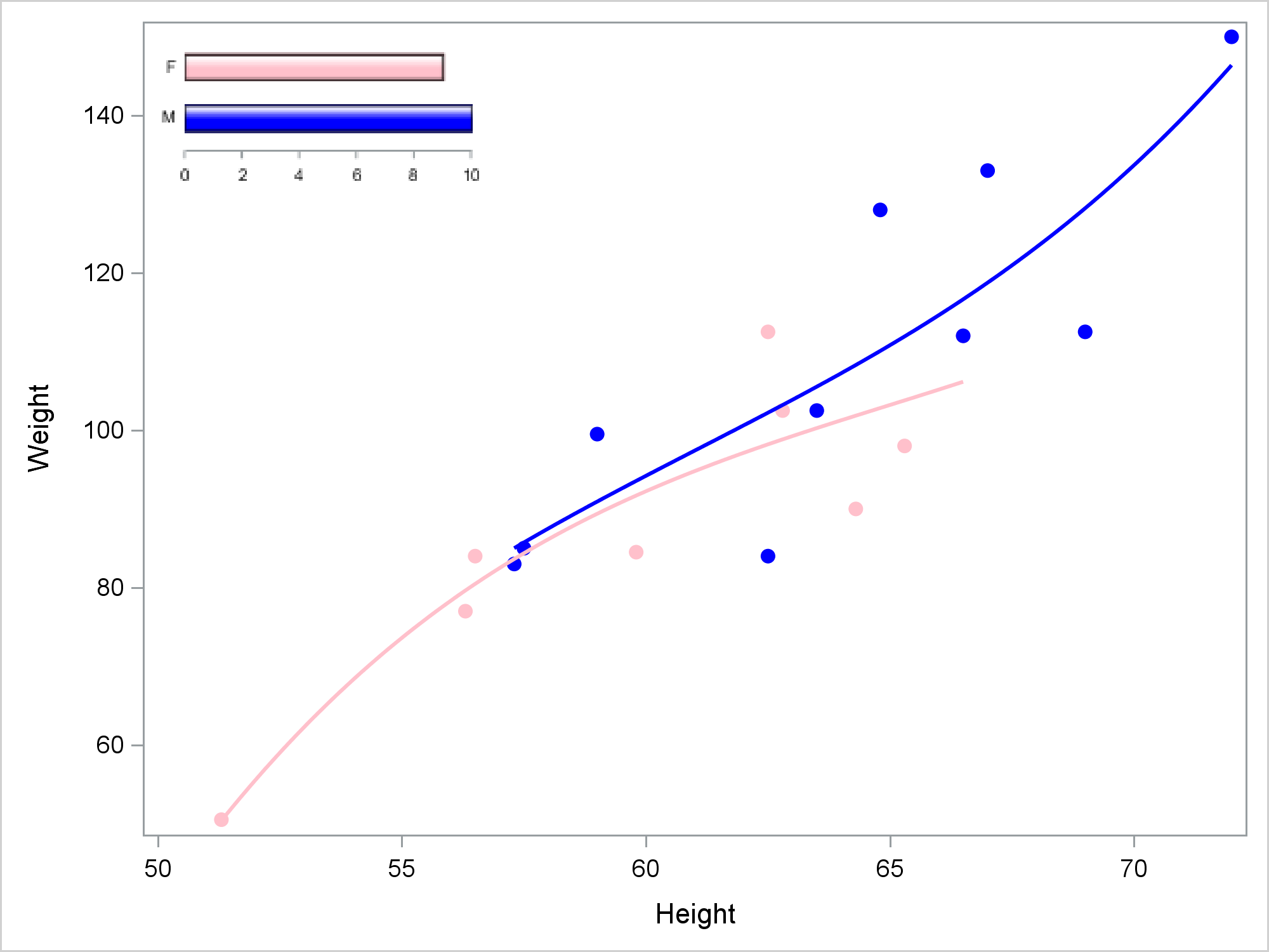
It has always been handy to add inset tables or legends inside a graph. Adding inset graphs adds an extra layer of flexibility to ODS Graphics. My first example uses PROC SGPLOT. The first step creates a bar chart that will become the inset. The second step creates an SG Annotation data set that inserts that bar chart into another graph. The third step creates a regression fit plot and inserts the bar chart. In all three examples, I make all graphs at 300DPI. I view the graphs in the HTML destination. Everything else, including the inset graphs, is suppressed. Of course, you are not required to do things this way nor should you as you develop code. I then further reduce the size of the graph when I display it in the other graph. In all cases, I took steps to suppress aspects of the inset graph, because multicomponent graphs rendered at small sizes are often not very elegant.
The first statements open the HTML destination, set the DPI, and set the location for the graphs. The image name for the first graph is set to Inset, and it is created at a small size. (The default in 480 by 640 pixels.)
ods html body='b.html' image_dpi=300 path="C:provide-your-folder-here"; ods graphics on / reset=all imagename="Inset" height=80px width=160px border=off; |
The ODS LISTING and ODS HTML statements combine to store the graph in a file and exclude it from the open HTML destination. The PROC SGPLOT step creates a bar chart with no border, no legend, and minimal axis components.
ods listing style=htmlblue;
proc sgplot data=sashelp.class noborder noautolegend;
   ods html exclude sgplot;
   styleattrs datacolors=(pink blue) datasymbols=(circlefilled);
   hbar sex / barwidth=0.5 group=sex baselineattrs=(thickness=0px)
              outlineattrs=(color=black) dataskin=gloss;
   yaxis display=(nolabel noticks noline);
   xaxis display=(nolabel) offsetmax=0;
run;
ods listing close; |
This step creates a simple SG Annotation data set that inserts the Inset.png file that the previous step made. The SG Annotation data set specifies the annotation function (image), the width (30%), the X and Y coordinates (1,99), the position (top left), the annotation drawing space (percentage of the graph wall), and the image name.
data anno;
   retain function "image" width 30 x1 1 y1 99 anchor "topleft"
          drawspace "wallpercent" image 'Inset.png';
run; |
This next step creates the graph shown near the top of the blog.
ods graphics on / height=480px width=640px reset=border imagename="Embedding"; proc sgplot data=sashelp.class sganno=anno noautolegend; styleattrs datacontrastcolors=(blue pink) datasymbols=(circlefilled); reg y=weight x=height / group=sex degree=3; run; |
Using two PROC SGPLOT steps is probably the easiest way to approach this problem. The next example uses an analytical procedure (it calls PROC LIFETEST twice) and modifies templates. The first step deletes any modified templates that might be left over from previous work (just to be safe) then writes the two templates of interest to two files.
proc template; delete Stat.Lifetest.Graphics.ProductLimitSurvival2 / store=sasuser.templat; delete Stat.Lifetest.Graphics.ProductLimitFailure / store=sasuser.templat; source Stat.Lifetest.Graphics.ProductLimitFailure / file='t'; source Stat.Lifetest.Graphics.ProductLimitSurvival2 / file='t2'; quit; |
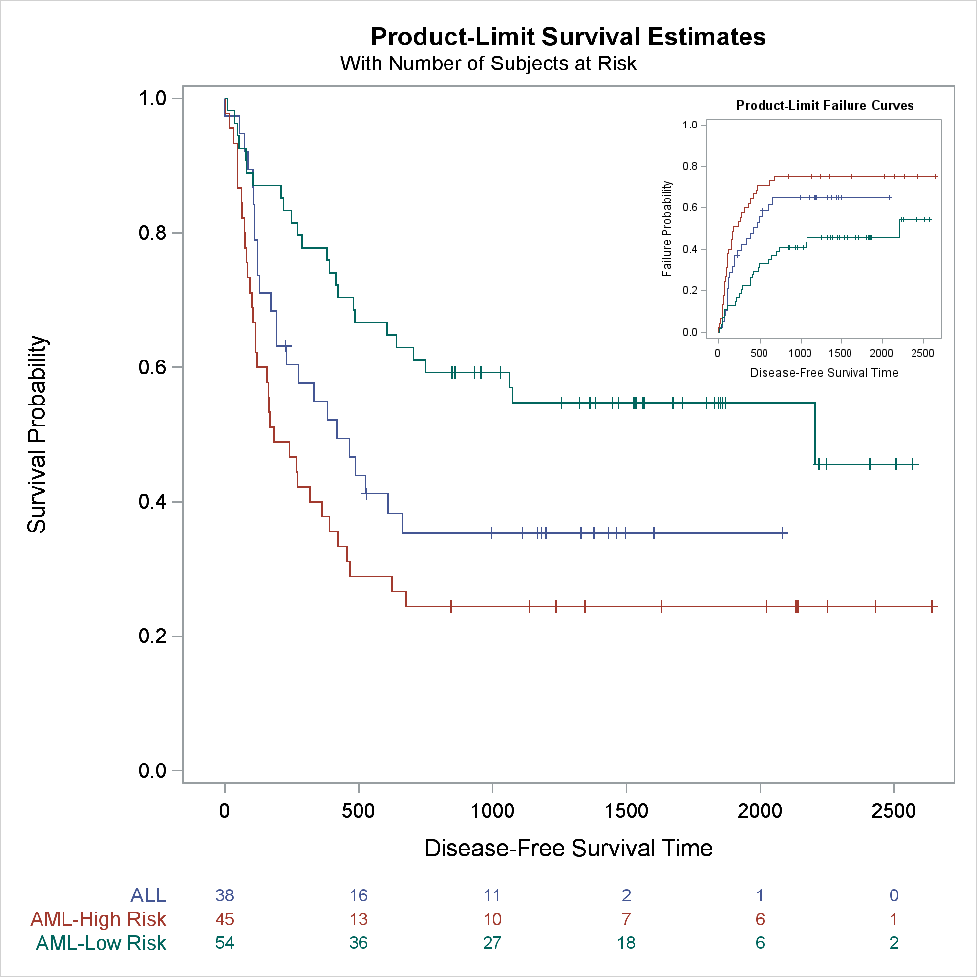
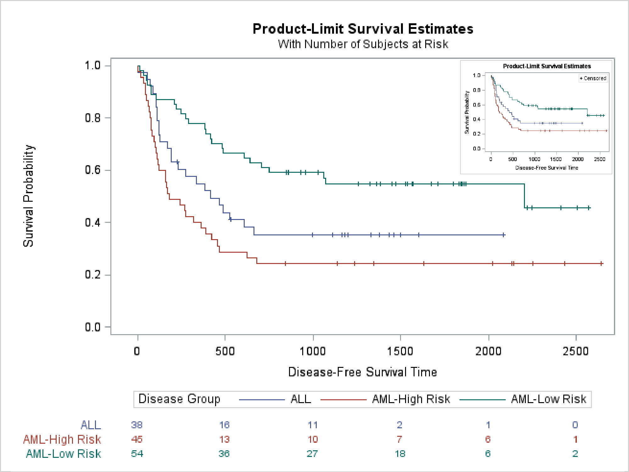
This example inserts a failure plot into the top right corner of a survival plot. The next step modifies the failure plot template to suppress the inset that contains the symbol for censored observations and the legend. (The third example shows a different way to suppress legends.) A DATA step and CALL EXECUTE modify the template and ensure that the SAS program produces reproducible results. (For more information about this type of template modification, see Advanced ODS Graphics Examples.) You can instead use an editor or any other means to modify the template. Note that I did not write this code in a vacuum. You must look at the template source code before writing the modification code. You can suppress legends by substituting names that do not appear elsewhere in the template.
data _null_;
   infile 't';
   input;
   if _n_ = 1 then call execute('proc template;');
   _infile_ = tranwrd(_infile_, 'discretelegend "Censored"',
                      'discretelegend "skipit"');
   _infile_ = tranwrd(_infile_, 'discretelegend "Failure"',
                      'discretelegend "skipit2"');
   _infile_ = tranwrd(_infile_, 'DiscreteLegend "Failure"',
                      'discretelegend "skipit2"');
   _infile_ = tranwrd(_infile_, 'entry "+ Censored"', ' ');
   call execute(_infile_);
run; |
The next step modifies the survival plot template. The SAS/STAT chapter Customizing the Kaplan-Meier Survival Plot illustrates many other ways to modify this plot.
data _null_;
   infile 't2';
   input;
   if _n_ = 1 then call execute('proc template;');
   if find(_infile_, 'layout overlay / xaxisopts') then lo + 1;
   if lo and index(_infile_, ';') then do;
      lo = 0;
      call execute(_infile_);
      _infile_ = 'drawimage "InsetI2.png" / width=38 x=99 y=99 anchor=topright
                  drawspace=wallpercent;';
      end;
   call execute(_infile_);
run; |
Statistical procedures such as PROC LIFETEST do not provide SG Annotation. However, you can add annotations by using a different method. The preceding step adds a DRAWIMAGE statement into the template after the end of each LAYOUT OVERLAY statement. There several other DRAW statements, and they correspond to the annotations that you can do by using SG Annotation in PROC SGPLOT.
The next step creates the failure plot at a reduced size using the modified failure plot template.
ods graphics on / imagename="InsetI2" height=300px width=300px border=off; ods listing style=htmlblue; ods html exclude all; proc lifetest data=sashelp.bmt plots=survival(failure); time T * Status(0); strata Group; run; ods html exclude none; ods listing close; |
The next step creates the survival plot at an expanded size using the modified survival plot template and the inset graph.
ods graphics on / reset=imagename reset=border height=640px width=640px; proc lifetest data=sashelp.bmt plots=survival(outside atrisk(maxlen=13)); ods select survivalplot; time T * Status(0); strata Group; run; |
The next step deletes the modified templates.
proc template; delete Stat.Lifetest.Graphics.ProductLimitSurvival2 / store=sasuser.templat; delete Stat.Lifetest.Graphics.ProductLimitFailure / store=sasuser.templat; quit; |
The last example creates two images and then uses SG annotation to insert them into an empty graph. Again, PROC LIFETEST is called twice, but this time the templates are not modified. This step creates a survival plot that displays an at-risk table.
ods graphics on / reset=all imagename='SurvivalI1' noborder; ods listing style=htmlblue; ods html exclude all; proc lifetest data=sashelp.bmt plots=survival(outside atrisk(maxlen=13)); ods select survivalplot; time T * Status(0); strata Group; run; |
This next step creates a smaller survival plot that has no at-risk table and no legend. The LEGENDAREAMAX=1 option suppresses the legend if it occupies more than 1% of the graph.
ods graphics on / reset=all imagename='SurvivalI2'
                  width=320px height=240px legendareamax=1;
proc lifetest data=sashelp.bmt plots=survival;
   ods select survivalplot;
   time T * Status(0);
   strata Group;
run;
ods html exclude none;
ods listing close; |
This step creates an SG Annotation data set that inserts the two images. The first is displayed at full size; the second is reduced.
data anno; retain function "image" anchor "topleft" drawspace "wallpercent"; length image $ 20; input x1 y1 width image $; datalines; 0 100 101 SurvivalI1.png 74 89 25 SurvivalI2.png ; |
This next step creates an input data set for PROC SGPLOT. If you want to only use SG Annotation to make the graph, you can make an invisible scatter plot of two corner points such as (1,1) and (-1,-1).
data corners; input x y @; datalines; 1 1 -1 -1 ; |
The following step displays both images (in the otherwise empty graph).
ods graphics on / reset=all imagename='SurvivalBoth'; proc sgplot data=corners sganno=anno noautolegend noborder; scatter y=y x=x / markerattrs=(size=0); yaxis display=none; xaxis display=none; run; |
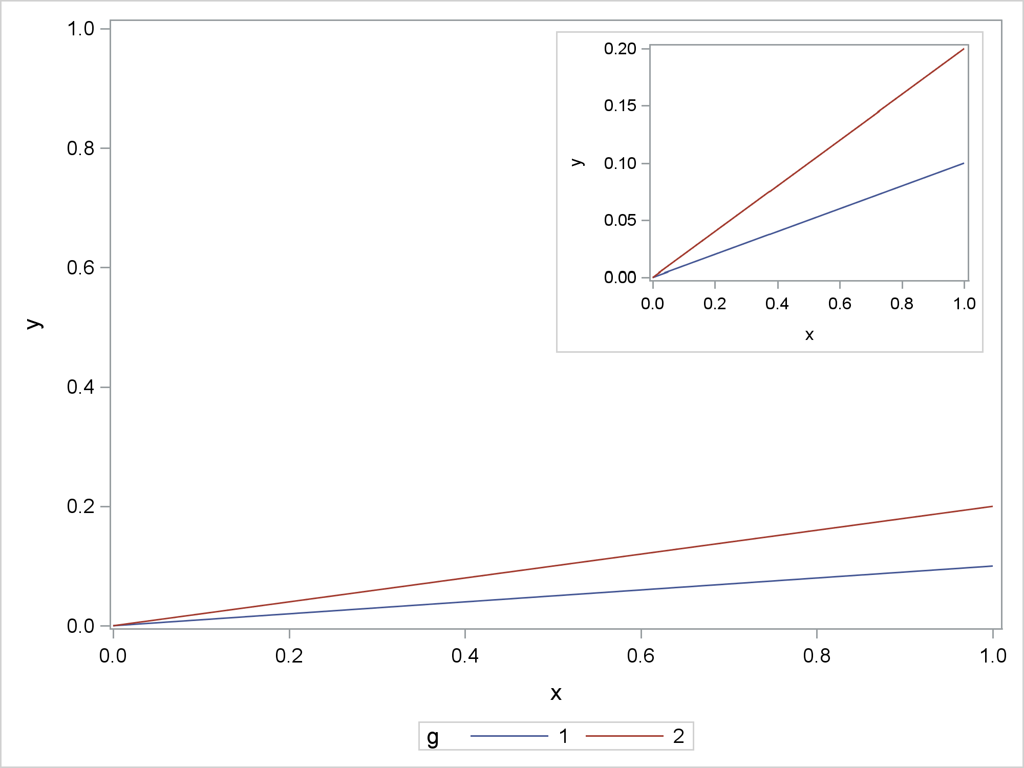
This last example is most similar to the example in the original question. The outer graph shows the full range of values on the Y axis. The inset graph is zoomed. While not shown here, the inset graph can show more details such as additional annotations. The difference between this example and the preceding examples involves the width. Here the dimensions are a constant proportion of the default dimensions. As long as you are using the default aspect ratio, you only need to specify the width. In the SG Annotation data set, the width is stated in pixels using the same proportion. This avoids any shrinking or expanding that might make the graphs less clear. This example also does not try to avoid separately displaying the inset graph.
data x;
   do x = 0 to 1 by 0.01;
      g = 1; y = 0.1 * x; output;
      g = 2; y = 0.2 * x; output;
      output;
   end;
run;

%let s = 2.4;
ods graphics on / reset=all imagename="Inset" width=%sysfunc(round(640/&s))px;
proc sgplot data=x noautolegend;
   series y=y x=x / group=g;* lineattrs=(thickness=2);
run;

data anno;
   retain function "image" width %sysfunc(round(640/&s)) widthunit "pixel"
          x1 50 y1 98 anchor "topleft"
          drawspace "wallpercent" image 'Inset.png';
run;

ods graphics on / reset=all;
proc sgplot data=x sganno=anno;
   series y=y x=x / group=g;
   yaxis min=0 max=1;
run;
ods html close; |
Of course you can modify the techniques shown here to combine PROC SGPLOT, PROC SGPANEL, and analytical procedures to display together two, three, or more graphs.