The Spring 2009 Foresight feature on assessing forecastability is a must-read for anyone who gets yelled at for having lousy forecasts. (It should also be read by those who do the yelling, but you’d have to be living in Neverland to believe that will ever happen.) As I promised in yesterday's guest blogging by Len Tashman, Editor of Foresight, here are a few comments on this topic.
Why is it that some things can be forecast with relatively high accuracy (e.g. the time of sunrise every morning for years into the future), while other things cannot be forecast with much accuracy at all, no matter how sophisticated our approach (e.g. calling heads or tails in the tossing of a fair coin)? Begin by thinking of behavior as having a structured, or rule-guided, or deterministic component, along with a random component. To the extent that we can understand and model the deterministic component, then (assuming we have modeled it correctly and the rule guiding the behavior doesn’t change over time) the accuracy of our forecasts is limited only by the degree of randomness.
Coin tossing gives a perfect illustration of this. With a fair coin, the behavior is completely random. Over the long term, our forecast (Heads or Tails) will be correct 50% of the time and there is nothing we can do to improve on it. Our accuracy is limited by the nature of the behavior – that it is entirely random.
While suffering from many imperfections (as Peter Catt rightly points out in his article), the Coefficient of Variation (CV) is still a pretty good quick-and-dirty indicator of forecastability in typical business forecasting situations. Compute CV based on sales for each entity you are forecasting over some time frame, such as the past year. Thus, if an item sells an average of 100 units per week, with a standard deviation of 50, then CV = standard deviation / mean = .5 (or 50%).
It is useful to create a scatterplot relating CV to the forecast accuracy you achieve. In this scatterplot of data from a consumer goods manufacturer, there are roughly 5000 points representing 500 items sold through 10 DCs. Forecast accuracy (0 to 100%) is along the vertical axis, CV (0 to 160% (truncated)) is along the horizontal axis. As you would expect, with lower sales volatility (CV near 0), the forecast was generally much more accurate than for item/DC combinations with high volatility.
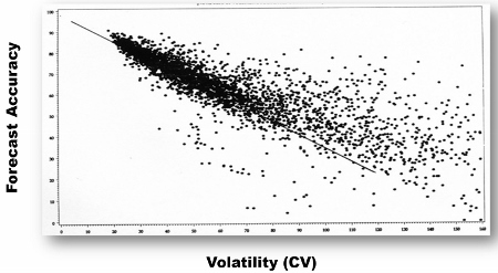
The line through this scatterplot is NOT a best fit regression line. It can be called the “Forecast Value Added Line” and shows the approximate accuracy you would have achieved using a simple moving average as your forecast model for each value of CV. The way to interpret the diagram is that for item/DC combinations falling above the FVA Line, this organization’s forecasting process was “adding value” by producing forecasts more accurate than would have been achieved by a moving average. Overall, this organization's forecasting process added 4 percentage points of value, achieving 68% accuracy versus 64% for the moving average. The plot also identifies plenty of instances where the process made the forecast worse (those points falling below the line), and these would merit further investigation.
Such a scatterplot (and use of CV) doesn’t answer the more difficult question – how accurate can we be? But I'm pretty convinced that the surest way to get better forecasts is to reduce the volatility of the behavior you are trying to forecast. While we may not have any control over the volatility of our weather, we actually do have a lot of control over the volatility of demand for our products and services. More about this another time…

13 Comments
Pingback: The “avoidability” of forecast error (Part 1) - The Business Forecasting Deal
Pingback: The "avoidability" of forecast error (Part 1) supplychain.com
Hi Mike,
Good article. It's been a long time since our days at Answer Think. I'm trying to introduce the CV concept in my current company to assess the forecastability of a product and ss. Looking at the literature for various cv forecastability thresholds. We find ourselves using the same ss calculation for all demand behavior. Products with high intermittent demand (thus high cv) is killing us (i.e.periods of product shortages and other periods of high inventory). Any suggestions?
ABC-XYZ Analyse would help you out
Pingback: Forecasting research project ideas - The Business Forecasting Deal
Mike,
What's the equation of the forecast value add line?
Jacob
Hi Jacob,
I once used FA = .98 - .63*CV as a VERY CRUDE approximation to the value added line for one company, based on the approximation of the FA of a moving average (naive) forecast at the various levels of volatility. I would advise AGAINST using something so crude and perhaps entirely inappropriate for the data at your organization.
I would suggest for each sku computing the FA you achieved, and the FA if you had used the naive "no-change" model and creating the scatterplot with both points for each SKU. This quickly becomes messy, so you'd want to experiment with visualizations. If you happen to come up with a good visualization, I'd love to share it in a blog post.
--Mike
HI Mike
i did not see scatterplot graph in this article. Where can i find it. Thanks
Hi Jacky -- not sure where the scatterplot (aka "Comet Chart") disappeared to, but I have re-inserted it into the post. You should be able to see it now. Thanks.
--Mike
Hi Mike,
Great article and analysis to assess the "forecastability" of time series. I have a question: is CV calculated using the training split or the test split of the time series? Or both? I assume the accuracy is computed using the training split only.
Thanks,
Mark
Hi Mark,
I've always used the most recent full year of available data (52 weeks or 12 months), although I suppose there is no harm in using a full 2 years or a full 3 years if you have it available. Using full yearly cycles is probably best, so as not to contaminate the CV calculation using only certain periods that are more or less volatile.
If you are using more granular time buckets, such as 15-minute increments which you might for electric utility demand or retail labor staffing, it might be more appropriate to calculate CV over a weekly cycle.
There is no hard rule here. Just calculate CV over the most appropriate time frame to represent what you are trying to forecast.
Thanks for the articles.
Can CV be applied to products with Sporadic/ intermittent demand?
For example, spares parts
look forward to your reply
Hi Shaun, sure you can still compute CV for intermittent demand, but your question raises an interesting issue. Many traditional forecasting performance metrics (such as MAPE) are inappropriate for intermittent data -- they become undefined due to 0 in the denominator. So it would become necessary to select an appropriate accuracy metric to compare CV to on a comet chart.
I personally do not consider intermittent demand a forecasting problem, but rather an inventory management problem. Yes, there are methods developed to forecast intermittent demand, but they are unlikely to result in highly accurate forecasts. So why spend the time on a futile endeavor? I would rather admit that we can't "solve" intermittent demand through forecasting, and instead focus on making good inventory decisions to meet customer needs in a fiscally responsible manner.
Another issue is raised by Steve Morlidge, who argues against using CV to measure the volatility of a series for forecasting purposes. He rightly points out that two series can have the same CV yet, because of the time sequence of the data points, have wildly different "forecastability" (my word).
For example, if 10 periods of demand are 1,2,3,...9,10 in that order, that looks like a steady upward trend. Compare that to the same 10 demands ordered randomly over the 10 periods, with no pattern at all.
Morlidge suggests computing the error of the (one period ahead) naive forecast over the data as a more useful indicator of volatility. Depending on the sequence of the data over time, this can give very different results from CV.