The Empirical Evidence
Steve Morlidge presents results from two test datasets (the first with high levels of manual intervention, the second with intermittent demand patterns), intended to challenge the robustness of the avoidability principle.
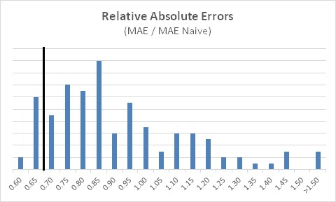
The first dataset contained one year of weekly forecasts for 124 product SKUs at a fast-moving consumer goods manufacturer. This company had a high level of promotional activity, with frequent manual adjustments to the statistical forecast. The histogram shows the ratio of the Mean Absolute Error (MAE) in their forecasts, compared to the MAE of the naive forecast. (Recall that when using MAE instead of MSE, the "unavoidability ratio" is at 0.7, as indicated by the vertical reference line.)
Results from the second dataset (880 SKUs across 28 months, with intermittent and lumpy demand) were similar.
The first observation is that relatively few items have the MAE ratio below 0.7 (and almost none below 0.5). Steve suggests that a ratio around 0.5 for MAE (less for MSE) may represent a useful lower bound benchmark for how good you can reasonably expect to be at forecasting.
The second observation is the large number of SKUs with a ratio above 1.0 -- meaning that the naive forecast was better! (In both datasets, over 25% of SKUs suffered this indignity!) These are examples of negative Forecast Value Added.
PLEASE TRY THIS AT HOME!
To further assess the usefulness of the avoidability concept, Steve welcomes participation from companies willing to further test and refine the approach. If you have data (suitably anonymized) you are willing to share, or have other questions or comments, you can reach him at steve.morlidge@satoripartners.co.uk.
At the very least, pull some of your own data and give the approach a try -- it's easy. Here is an example of the calculation, for one SKU over 52 weeks. All you need is the Forecast and the Actual over the choosen time period, and it is easy to recreate the naive (random walk) forecast from the Actuals:
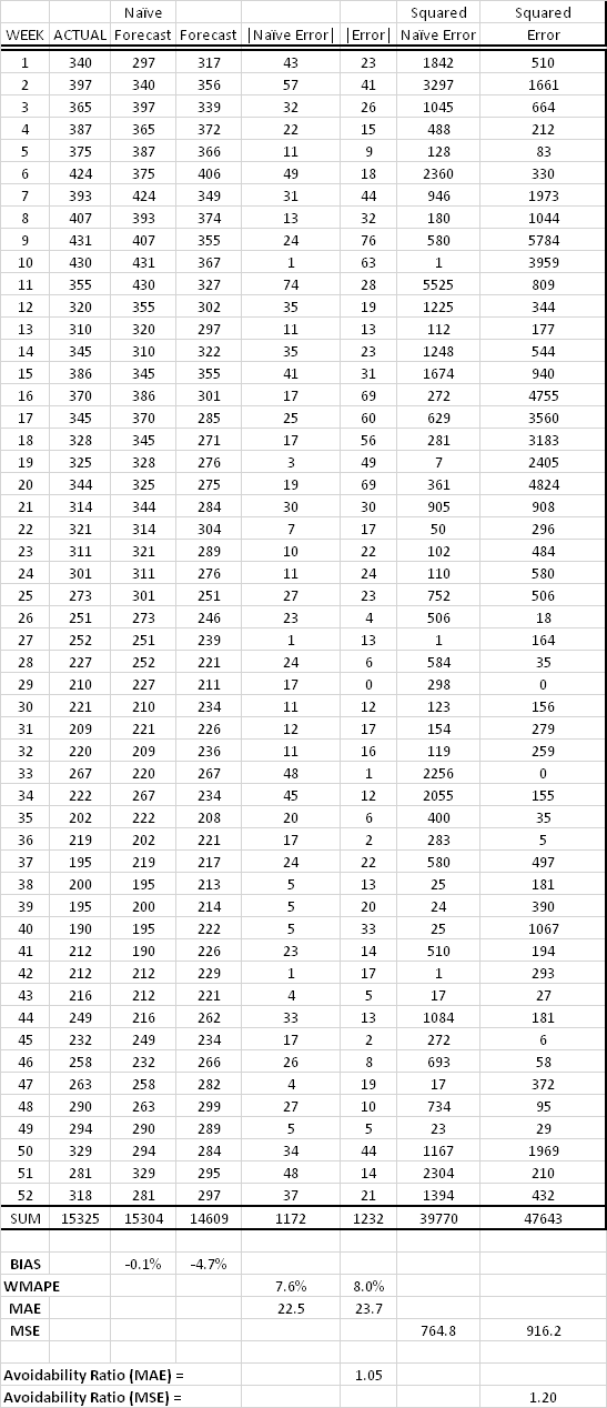
In this example the avoidability ratio was > 1.0 (using either MAE or MSE), indicating a very poor forecast that was actually worse than a naive forecast, and was also significantly biased (averaging nearly 5% too low). A good (value adding) forecasting process will deliver ratios < 1.0, and (we hope) get down below 0.7 for MAE (or 0.5 for MSE).

6 Comments
Hi Mike,
I've been following Steve Morlidge's work and was so happy to run across your blog walking through the maths.
I'm "trying this at home" and strugling with the Squared Naive Error and Squared Error columns in your example. Is there an error in your squaring formula? Given the first week's absolute naive error of 43, I was expecting the Squared naive error to be 1849. Likewise for the absolute error and squared values. I expected 23 & 529.
Is this a mistake in the example table or am I missing something?
Thanks in advance for your response,
Lawrence
Hi Lawrence, thanks for the note, and glad to hear you are trying this at home!
To mildly disguise the original data and keep a clean look in the table, I divided the original data by a factor and am not showing the decimal places. That is why the squared values look a little off. (Looking back, I should have rounded everything to integers before squaring, and thus avoided creating this confusion.)
I understand that Steve Morlidge will soon be publishing some additional work on this topic. I'm looking forward to that, and will cover it here in the blog. Thanks,
--Mike
Pingback: Q&A with Steve Morlidge of CatchBull (Part 1) - The Business Forecasting Deal
Pingback: SAS/Foresight Q4 webinar: Avoidability of Forecast Error - The Business Forecasting Deal
Hello Mr Gilliland.
The forecast that you evaluate is in LAG 0 or LAG1? Coud one evaluate with this procedure longers LAGS?
Hi Leopoldo, yes you could do the evaluation over longer lags. This would be appropriate when there is longer supply lead time, so you evaluate the forecast you made at the lead time.
In the blog example, I compared the latest forecast to the naive "no change" model based on prior week's actuals.
If, for example, there is a 3-week supply lead time, then you would compare the 3-week ahead forecast to the naive forecast (which is the actual from 3 weeks prior).