In this guest blogger post, Udo Sglavo of the Advanced Analytics Division of SAS shows how to conduct time series cross-validation using SAS Forecast Server.  Udo replicates the example from Rob J Hyndman's Research Tips blog.

Replicating the Example

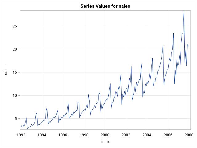
In order to replicate the example in Hyndman's blog, the example data set A10 (“Monthly sales of anti-diabetic drugs in Australia”) was ported from R to SAS using a CSV file and plotted:

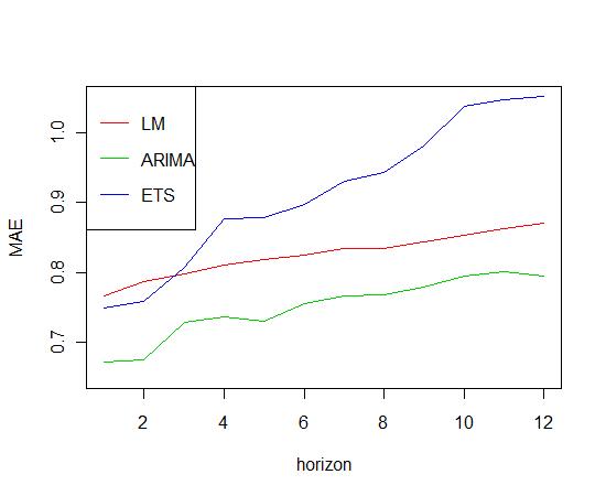
Hyndman applies time series cross-validation and compares 1-step, 2-step, …, 12-step forecasts using the Mean Absolute Error (MAE). He writes: “Here I compare (1) a linear model containing trend and seasonal dummies applied to the log data; (2) an ARIMA model applied to the log data; and (3) an ETS model applied to the original data.” Furthermore Hyndman suggests using 60 observations of the data as a minimum to estimate the model parameters.

In SAS High-Performance Forecasting, these models can be implemented using the following code (note that a selection list containing only one model is created, due to cross-validation):

PROC HPFARIMASPEC
      /* LOG(Y) = P=( 1 2 3 ) D=(s) Q=( 1 )( 1 )s  */
      MODELREPOSITORY = work.temp SPECNAME=ARIMA301011;
      FORECAST TRANSFORM = LOG DIF = ( s ) P = ( 1 2 3 ) Q = ( 1 ) ( 1 )s;
run;
 
PROC HPFSELECT
      /* Model Selection List */
      MODELREPOSITORY = work.temp SELECTNAME=ARIMA;
      SPEC ARIMA301011;
run;
 
PROC HPFARIMASPEC
      /*LOG(Y) =   LINEAR + SEASONAL*/
      MODELREPOSITORY = work.temp SPECNAME=LOGLINEARSEASONALDUMMIES;
      FORECAST SYMBOL = Y TRANSFORM = LOG;
      INPUT PREDEFINED = LINEAR TRANSFORM = NONE;
      INPUT PREDEFINED = SEASONAL TRANSFORM = NONE;
run;
 
PROC HPFSELECT
      /* Model Selection List */
      MODELREPOSITORY = work.temp SELECTNAME=LOGLIN;
      SPEC LOGLINEARSEASONALDUMMIES;
run;
 
PROC HPFESMSPEC
      /* Multiplicative Winter’s Method */
      MODELREPOSITORY = work.temp SPECNAME=WINTERS;
      ESM METHOD = WINTERS;
run;
 
PROC HPFSELECT
      /* Model Selection List */
      MODELREPOSITORY = work.temp SELECTNAME=ESM;
      SPEC WINTERS;
run;

To implement cross-validation using SAS High-Performance Forecasting SAS macros were used. Similar to what Hyndman describes data points at the end of the series were left out to calculate MAE “manually” by using the BACK= option of SAS High-Performance Forecasting. Again, instead of using the HOLDOUT= option provided cross-validation as suggested by Hyndman was used to pick the best performing model. Note that some of the parameters passed to HPFENGINE call are macro variables.

PROC HPFENGINE DATA=a10 OUT=_null_
     OUTFOR=&model._&i.(where=(date ge "&end2."d) keep=date error)
     repository=work.temp GLOBALSELECTION=&model BACK=&lead LEAD=&lead;
     ID date INTERVAL=month START="&start"d END="&end."d;
     FORECAST sales;
run;

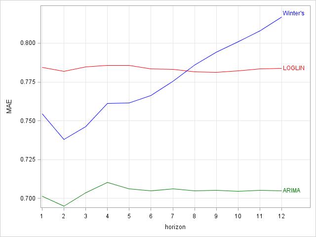
Finally the results of each of the 12 runs for each of the lead times are plotted, to replicate the graphic provided by Hyndman:

PROC SGPLOT DATA=plot NOAUTOLEGEND;
      xaxis type=discrete grid;
      yaxis label="MAE" grid;
      series x=horizon y=mae1 /lineattrs=(color=green) curvelabel="ARIMA";
      series x=horizon y=mae2 /lineattrs=(color=red) curvelabel="LOGLIN";
      series x=horizon y=mae3 /lineattrs=(color=blue) curvelabel="Winter's";
run;

Note that the resulting plot shows some differences compared to the one by Hyndman. This might be due to differences in the computation methods for the model parameters. In general the result is the same. Using time series cross-validation the ARIMA model outperforms the 2 other methods for all 12 lead times, so it should be the preferred forecasting method for the data at hand.

Hyndman:

SAS:

Hyndman writes: “The code is slow because I am estimating an ARIMA and ETS model for each iteration.” – the SAS code is also very computing intensive and takes about 2.5 minutes to run in batch using SAS 9.3 on a laptop with 4 GB of RAM and 2,67 GHz on a 64-bit OS.

(Full SAS code is available upon request from udo.sglavo@sas.com)

In Part 2, we'll look at out-of-sample testing and draw some conclusions.